Global Health for Engineers

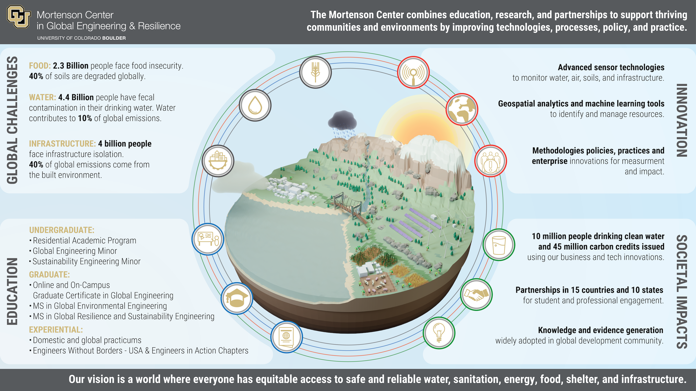
Mortenson Center in Global Engineering

University of Colorado Boulder

This is the Mortenson Center in Global Engineering at CU Boulder. Our mission is to improve the effectiveness of humanitarian engineering programs through education, research, and partnerships. We work across water, sanitation, energy, and public health — always with an emphasis on rigorous evidence and community-driven design.

Course Structure

An introduction to the professional field of Global Health, particularly focused on the areas of global health that engineers often contribute to – i.e. community environmental health. In a short course, we won't have time to touch on things like health systems organization but there are many resources for additional learning.

We will be reading published peer reviewed studies of global health interventions – learning how to search for, read and analyze these kinds of studies is fundamental to being conversant in the field of global health. Many of these papers have engineers as co-authors.

This class is also an opportunity for group and 1:1 discussion. I am happy to meet with each of you individually to discuss career objectives and networking.

Class will be heavy on case studies, with student-led facilitation.

All readings posted in Canvas. Textbook is self-paced with online Canvas quizzes.

See Canvas Syllabus for link to class schedule.

The backbone of this course is reading real peer-reviewed studies — the same literature that informs policy and program design in global health. We will focus on community environmental health, which is the area where engineers have the most direct impact. I also want this to be a conversation, so come prepared to discuss the readings and bring your own questions about career paths in this field.

Evan Thomas

Professor

Environmental Engineering Program
Civil, Environmental and Architectural Engineering Dept.
Aerospace Engineering Sciences Department

Mortenson Endowed Chair in Global Engineering

Director, Mortenson Center in Global Engineering

University of Colorado Boulder

PhD, Aerospace Engineering Sciences, 2009
MS, Aerospace Engineering Sciences, 2006
BS, Aerospace Engineering Sciences, 2005
BS, Broadcast Journalism, 2005

Oregon Health and Science University

MPH, Master in Public Health, 2014

Fletcher School at Tufts University

Global MBA, 2022

NASA Johnson Space Center, Aerospace Engineer, 2004-2010

Portland State University, Assistant/Associate Professor, 2010-2018

Virridy Inc, Founder and CEO, 2012 – Present

Manna Energy Limited / DelAgua Health, Founder, COO, 2007-2016

~80 journal articles, 10 patents, professional work in 16 countries

A bit about my background — I started in aerospace engineering at NASA, which might seem unrelated to global health, but the systems thinking and sensor design skills transferred directly. I went back for a Master of Public Health because I realized the engineering was only useful if grounded in epidemiology and health evidence. I have founded companies working on water quality monitoring and carbon finance for health, and I have worked in about 16 countries across Africa, Asia, and Latin America.

The Global Health Architecture

Understanding the major organisations and funding mechanisms that shape global health policy, programs, and research.

Multilateral Organisations

WHO — sets norms, coordinates response, technical guidance
UNICEF — child health, nutrition, immunisation, WASH
World Bank — health system financing and development loans

Public-Private Partnerships

Gavi — vaccine access for 1B+ children since 2000
Global Fund — AIDS, TB, and malaria ($60B+ disbursed)
CEPI — epidemic preparedness and vaccine R&D

Bilateral Aid Agencies

USAID (US) — largest bilateral health donor (~$10B/yr)
FCDO (UK), GIZ (Germany), JICA (Japan)
PEPFAR — US HIV/AIDS programme, 25M+ on treatment

Philanthropic & Research

Gates Foundation — largest private funder (~$7B/yr)
Wellcome Trust — biomedical research in LMICs
MSF / Red Cross — frontline emergency response

The next section examines what happens when this architecture is disrupted.

Before we can understand what is happening right now, you need to know the ecosystem. These organizations — WHO, UNICEF, the World Bank, Gavi, the Global Fund, USAID, the Gates Foundation — are the architecture that global health runs on. Each plays a distinct role, from setting norms and coordinating outbreak response to financing vaccines and running bilateral aid programs. Understanding who does what is essential because when any part of this system breaks, the consequences ripple across the entire landscape.

Context

The Current State of Global Health

2025–2026: A period of unprecedented disruption to global health infrastructure.

Now we transition to something that is not in any textbook yet because it is happening right now. The global health architecture we just described is being disrupted in ways that are unprecedented in the modern era. I want you to understand these changes not as abstract policy debates, but as concrete events with measurable consequences for health outcomes around the world.

USAID Shutdown

Timeline

Jan 20, 2025: Executive Order freezing all foreign assistance funds for 90 days, including PEPFAR
March 2025: Termination of 83% of USAID's 6,300 global initiatives
Staff cut from 10,000 to 15 personnel
Feb 2026: Congress passed $50B foreign aid bill to begin reinvestment

Projected Impact

9.4 million additional deaths projected by 2030 (The Lancet)
500,000–1,000,000 lives lost in 2025 alone (Center for Global Development)
2.3 million people on antiretroviral treatment lost support
12.5–17.9 million additional malaria cases projected
2.4 million people in Yemen lost food assistance

This is not abstract. In January 2025, an executive order froze all foreign assistance, and within weeks 83 percent of USAID's programs were terminated. The staff went from 10,000 to 15. The Lancet projects 9.4 million additional deaths by 2030 as a result. Think about that — 2.3 million people on antiretroviral therapy lost their supply chain overnight, and Congress did not pass a reinvestment bill until early 2026.

US Withdrawal from the WHO

What Happened

Jan 20, 2025: Executive order giving one-year notice of withdrawal
Jan 22, 2026: US formally withdrew from the WHO
US historically contributed ~15% of WHO's total budget (~$1.28 billion annually)
WHO cutting ~2,371 staff (25% reduction) by mid-2026

Consequences for Global Health

Global Influenza Surveillance and Response System (GISRS) disrupted — seasonal flu vaccine formulation at risk
50-country disease surveillance network dismantled
Emergency outbreak response time reverted from <48 hours to >2 weeks
Pandemic preparedness infrastructure weakened

The US contributed about 15 percent of WHO's budget — over a billion dollars a year. When the US formally withdrew in January 2026, WHO had to cut a quarter of its staff. The consequences are tangible: the flu vaccine formulation process depends on the Global Influenza Surveillance network, outbreak response times have gone from under 48 hours to over two weeks, and a 50-country disease surveillance network was dismantled.

EPA Rollbacks, CDC Cuts & Domestic Health

EPA Regulatory Rollbacks

31 climate, air, and water pollution regulations rolled back
Emissions reporting requirements for CO₂, methane, and other GHGs eliminated
Coal-fired power plant emission restrictions dismantled
Air pollution-related deaths projected to increase by tens of thousands per year

CDC Budget & Workforce Cuts

Proposed 53% budget reduction for FY 2026
~25% of CDC workforce cut by end of 2025
42,000 jobs lost nationwide if proposed cuts adopted
60+ CDC programs eliminated, including global HIV/AIDS prevention and global immunization
Morbidity and Mortality Weekly Report (MMWR) staff fired

Surveillance & Preparedness

12+ health tracking programs eliminated (deaths, disease trends)
Disease detectives, outbreak forecasters, and data offices cut
Public Health Emergency Preparedness funding cut 52%
Weakened capacity for early detection, outbreak investigation, and pandemic preparedness

Global health starts at home. The EPA rolled back 31 climate, air, and water regulations. The CDC is facing a proposed 53 percent budget cut and has already lost a quarter of its workforce. The MMWR — the main publication for disease surveillance data in the US — lost its staff. When we lose the ability to track disease domestically, it affects our ability to detect outbreaks before they become global problems.

Implications for Global Health Engineers

Funding Landscape Shift

Traditional USAID-funded pathways for global engineering projects are disrupted. New funding models needed — carbon credits, private sector, multilateral alternatives.

Surveillance Gaps

Engineers working in water, sanitation, and environmental monitoring face a world with weaker disease surveillance and slower outbreak response.

Domestic & Global Nexus

EPA rollbacks demonstrate that environmental health is not just a developing-country issue. Air and water quality challenges affect communities everywhere.

Local Capacity Building

With reduced external support, building local technical and institutional capacity is more critical than ever for sustainable health outcomes.

Data & Evidence

Loss of federal data collection increases the importance of independent monitoring, sensor networks, and digital MRV systems.

Discussion

How should the global health engineering community respond to these changes? What role can universities and the private sector play?

So what do we do about all of this? This is a discussion slide, and I want to hear your ideas. The traditional USAID-funded pathway for engineering projects abroad is disrupted, so we need to think about alternative funding models like carbon credits and private sector partnerships. We also need to think about building local capacity so programs are not dependent on any single donor, and about the role of independent monitoring and sensor networks when government data collection is weakened.

Section

Intro to Global Health
Part 1 - Overview

Now we shift from the current disruptions to the foundational concepts you need to understand global health. This section covers what global health actually is, what determines whether people are healthy or sick, and the key frameworks for thinking about health at the population level. These are the concepts that will underpin everything else in the course.

What is Global Health?

"An area for study, research, and practice that places a priority on improving health and achieving equity in health for all people worldwide. Global health emphasizes transnational health issues, determinants, and solutions; involves many disciplines within and beyond the health sciences and promotes interdisciplinary collaboration; and is a synthesis of population-based prevention with individual-level clinical care."

— Consortium of Universities for Global Health

Overview Objectives

Define the determinants, including social and economic, that impact health.

Highlight the differences in disease and life expectancy between high- and low-income countries.

Identify some of the dynamics in developing countries that impact health trends.

Key Concepts

The determinants of health

The measurement of health status

The importance of culture to health

The global burden of disease

Key risk factors for health problems

Organisation of health systems

Disciplines: Public Health · Public Policy · Medicine · Social Sciences · Behavioural Sciences · Law · Economics · History · Engineering · Biomedical Sciences · Environmental Sciences · Anthropology

This is the formal definition from the Consortium of Universities for Global Health. The key words to notice are equity, transnational, interdisciplinary, and population-based. Global health is not just tropical medicine — it is about understanding why health outcomes differ across and within countries, and engineering is explicitly one of the contributing disciplines. Our objectives for this section are to define health determinants, highlight disparities between high- and low-income countries, and identify the dynamics that drive health trends.

Disease & Determinants of Health

Examples of disease that disproportionately impact developing countries

Malaria
Diarrhea
Pneumonia
HIV / Aids

99% of the children under the age of 5 who die every year lived in developing countries.

Determinants of Health

Genetics
Age
Gender
Lifestyle choices
Community influences
Income status
Geographical location
Urbanization
Climate Change
Governance
Culture
Environmental factors
Work conditions
Education
Access to health services

On the left we have diseases that disproportionately kill people in developing countries — malaria, diarrhea, pneumonia, HIV. On the right, the determinants of health — the factors that explain why these diseases cluster where they do. The statistic that should stick with you is that 99 percent of children under 5 who die each year lived in developing countries. That is not because of genetics — it is because of the determinants on the right side of this slide.

Multi-sectoral Dimension of the Determinants of Health

Malnutrition

More susceptible to disease and less likely to recover

Cooking with wood and coal

Lung diseases

Poor sanitation

More intestinal infections

Poor life circumstances

Commercial sex work and STIs, HIV/AIDS

Advertising tobacco and alcohol

Addiction and related diseases

Rapid growth in vehicular traffic

Road traffic accidents

Health is not just a medical issue — it is multi-sectoral. Malnutrition makes you more susceptible to disease and less likely to recover. Cooking with wood and coal causes lung disease. Poor sanitation leads to intestinal infections. Tobacco advertising drives addiction. Rapid growth in vehicular traffic causes road injuries. As engineers, several of these sectors are areas where we can design interventions — clean cooking, sanitation, safe transportation infrastructure.

One Health — Zoonotic Disease at the Human-Animal-Environment Interface

Emerging Zoonoses

75% of emerging infectious diseases are zoonotic. COVID-19, mpox, Ebola, avian influenza, and MERS all crossed from animals to humans.

Environmental Drivers

Deforestation, urbanization, intensive agriculture, and climate change increase contact between wildlife, livestock, and humans — creating spillover opportunities.

Engineering Role

Water and sanitation engineers work at the human-environment boundary. Wastewater surveillance, safe animal husbandry infrastructure, and environmental monitoring are engineering contributions to One Health.

One Health is the framework that recognizes human, animal, and environmental health are interconnected. Seventy-five percent of emerging infectious diseases are zoonotic — they crossed from animals to humans. COVID-19, Ebola, avian influenza — all zoonotic. The environmental drivers are deforestation, urbanization, intensive agriculture, and climate change. As water and sanitation engineers, we work right at that human-environment boundary, and wastewater surveillance is increasingly an important tool for detecting outbreaks.

Governance & Armed Conflict

Governance

Governance has a direct impact on socioeconomic status, health inequalities, and development

Allocation of Resources
Control of policy
Trade agreements
Regional politics
Abuse of power
Education

Armed Conflict

The Results:

Disparities over resources and power
Broken relationship with neighboring countries
Lack of development
Inequality along race/gender lines
Resources diverted from health care to support conflict
Displacement

Health Implications:

Malnutrition
Diarrhea
Respiratory infections
AIDS
Extreme poverty
Negative long-term effects on health

Governance and armed conflict are health determinants that engineers often do not think about, but they are critical. How a government allocates resources, controls policy, and manages trade directly affects health outcomes. Armed conflict diverts resources from healthcare, displaces populations, and creates the conditions for malnutrition, diarrhea, respiratory infections, and extreme poverty. If you are designing an engineering intervention, you need to understand the governance and conflict context you are working in.

Section

Intro to Global Health
Part 2 – Global Burden of Disease

Now we move to the data. This section is about quantifying the global burden of disease — how many people are getting sick and dying, from what causes, and where. I want you to develop an intuition for the numbers and the geographic patterns, because evidence-based engineering requires understanding the scale and distribution of the problems we are trying to solve.

Explore the Data

Interactive tools for exploring the Global Burden of Disease: GBD Compare | SDG Visualizations | Our World in Data

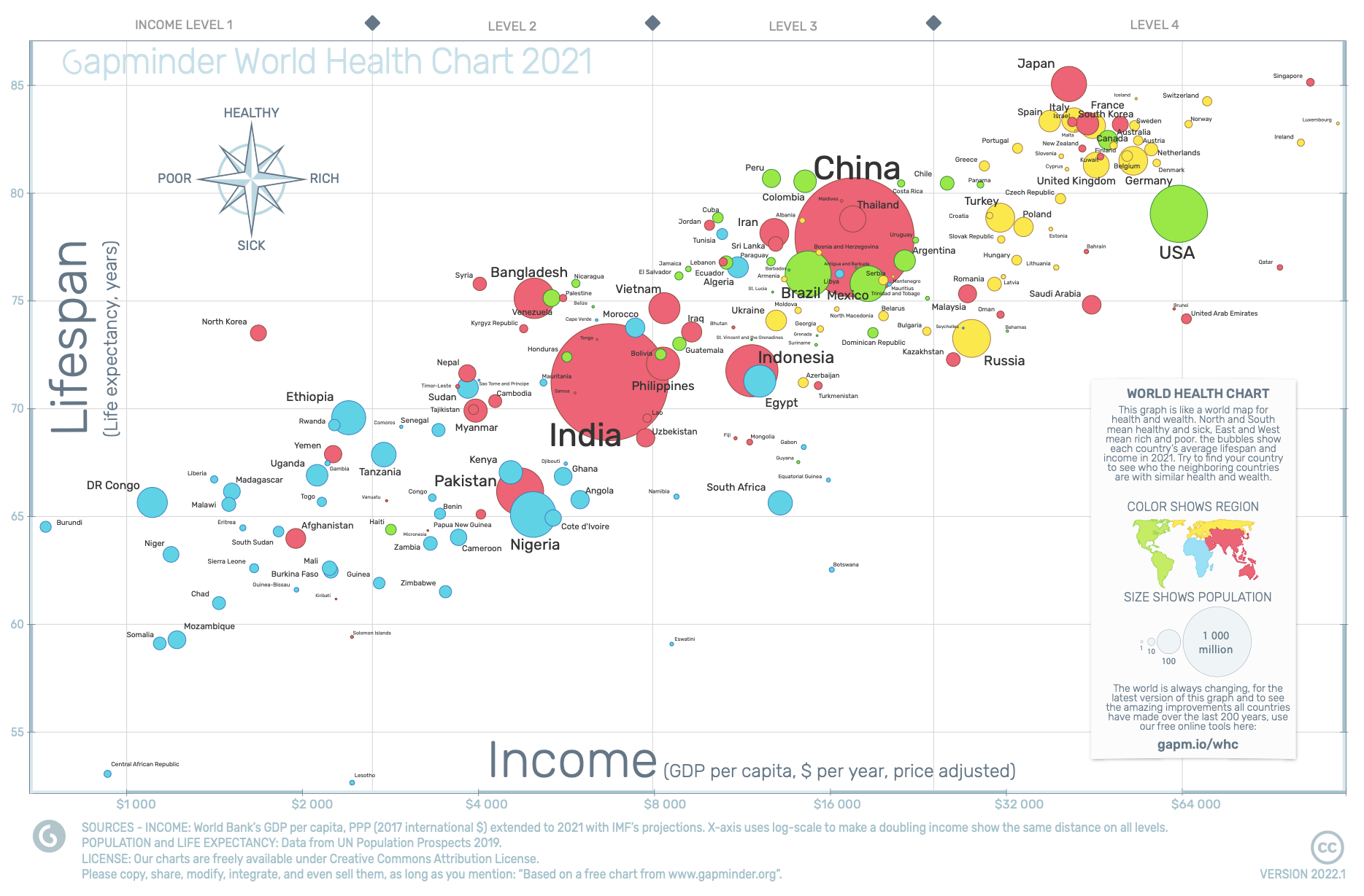
These are the interactive tools I want you to explore outside of class. The IHME GBD Compare tool lets you visualize the global burden of disease by cause, age, sex, and country. Our World in Data is excellent for trends over time. And Gapminder, which Hans Rosling made famous, shows the relationship between health and income in a way that challenges many assumptions. The chart you see here is the classic health-and-wealth bubble plot.

Health & Income of Nations

Life expectancy vs. GDP per capita. Bubble size = population, color = region. Source: World Bank / UN, 2023.

This is the Gapminder visualization showing life expectancy versus income per capita, with bubble size representing population and color representing world region. The key insight is the strong relationship between wealth and health — richer countries tend to have higher life expectancy. But there is enormous variation, and some countries punch well above or below their income level, which tells us that policy and governance matter beyond just economic development.

Global Mortality Among Children Under 5

Total deaths by cause, 1990–2021. Sources: IHME GBD 2021, UNICEF IGME 2024, WHO Global Health Estimates.

This chart shows the major causes of death in children under 5 from 1990 to 2021. The good news is that nearly every cause has declined substantially — lower respiratory infections dropped from over 10 million to under 3 million deaths. But notice malaria ticked back up recently, and the total is still nearly 5 million children per year. These are largely preventable deaths from causes we know how to address with existing technologies and interventions.

Child Mortality in Sub-Saharan Africa

Total under-5 deaths by cause, 1990–2021. Sources: IHME GBD 2021, WHO Africa Region, UNICEF IGME 2024.

When we zoom into Sub-Saharan Africa specifically, you can see that this region bears a disproportionate share of the global burden. Malaria is the leading killer here, and it actually increased in the early 2000s before control efforts brought it down, though it has risen again recently. Sub-Saharan Africa accounts for the majority of child mortality worldwide, and understanding why requires looking at the interaction of poverty, weak health systems, and environmental conditions.

Extreme Poverty by Region

People living below $2.15/day (2017 PPP). Sub-Saharan Africa is the only region where absolute numbers are rising. Source: World Bank, 2024. By 2030, 9 in 10 people in extreme poverty will live in Sub-Saharan Africa.

This chart tells one of the most important stories in global health. East Asia, driven largely by China, saw an extraordinary decline in extreme poverty — from over a billion people to about 29 million. South Asia has also made remarkable progress. But Sub-Saharan Africa is the only region where the absolute number of people in extreme poverty is rising. By 2030, nine out of ten people living in extreme poverty will be in Sub-Saharan Africa. This is the geographic concentration that drives most of the disease burden we have been looking at.

Per Capita CO₂ Emissions

High-income countries have the highest per capita emissions, while low-income countries with the greatest disease burden contribute the least.

Now look at who is causing climate change versus who is bearing the burden of disease. High-income countries have the highest per-capita CO2 emissions, while low-income countries with the greatest disease burden contribute the least. This is the equity dimension of climate and health — the populations least responsible for emissions are the most vulnerable to their health consequences, from heat stress to vector-borne disease expansion to food insecurity.

Global Burden of Disease

DALYs per 100,000 from all causes. Sub-Saharan Africa and South Asia bear the highest disease burden.

This map shows DALYs — disability-adjusted life years — per 100,000 people from all causes. The darker regions represent higher disease burden. You can clearly see that Sub-Saharan Africa and parts of South Asia have dramatically higher burdens than the rest of the world. DALYs capture both premature death and years lived with disability, so this is a comprehensive measure of health loss.

Undernourishment

Share of population with insufficient caloric intake. Malnutrition is a key determinant of susceptibility to disease.

Undernourishment — insufficient caloric intake — is both a consequence of poverty and a driver of disease. Malnourished individuals are more susceptible to infections and less likely to recover. This map shows the geographic distribution, and it closely mirrors the poverty and disease burden maps we have been looking at. Malnutrition is a cross-cutting determinant that amplifies nearly every other health challenge.

Child Mortality — Causes of Death Under 5

4.9 million children under five died in 2024 — over 13,400 every day. Nearly 90% in LMICs.

The causes of death differ dramatically between high-income and low-income countries.

Low-Income Countries

High-Income Countries

Sources: IHME GBD 2021, UNICEF IGME 2024, WHO Global Health Estimates. Shares are % of total under-5 deaths.

Here we compare causes of child mortality between low-income and high-income countries side by side. In low-income countries, malaria, pneumonia, and diarrheal diseases dominate — these are infectious diseases driven by environmental conditions that engineers can address. In high-income countries, congenital birth defects and neonatal complications are the leading causes, because the infectious disease burden has been largely eliminated through water, sanitation, vaccination, and health system infrastructure.

Disease Burden

Communicable & Non-Communicable Diseases

Now we are going to do deep dives on specific diseases — both communicable diseases like malaria and HIV, and the growing burden of non-communicable diseases. For each disease, I want you to think about the transmission pathway, the geographic distribution, and what engineering interventions exist or could be developed.

Communicable Diseases — Definition & Transmission

"Any condition transmitted directly or indirectly to a person from an infected person, animal, vector, or through the inanimate environment."

Direct transmission

Blood-borne / sexual — HIV, Hepatitis B & C
Inhalation — Tuberculosis, influenza, anthrax
Food-borne — E. coli, Salmonella
Contaminated water — Cholera, rotavirus, Hepatitis A

Indirect transmission

Vector-borne — malaria, onchocerciasis, trypanosomiasis
Fomites — contaminated objects and surfaces
Zoonotic — animal-to-human (avian influenza, Ebola, MERS)

Key drivers of emergence (IOM)

Globalisation — affordable international air travel, increased trade
Microbial adaptation and drug resistance
Breakdown of public health capacity
Changing demographics, behaviour, land use, and urbanisation

A communicable disease is any condition transmitted directly or indirectly from an infected person, animal, vector, or through the environment. The transmission routes matter for engineering because they tell us where to intervene — water treatment for cholera, ventilation for TB, vector control for malaria, food safety systems for E. coli. The key drivers of emergence identified by the Institute of Medicine include globalization, microbial adaptation, and breakdown of public health capacity — that last one is particularly relevant given what we discussed about USAID and WHO.

Impact of Communicable Diseases

Disease Burden

CDs account for ~30% of the global burden of disease and ~60% in Africa
40% of the disease burden in LMICs; disproportionately affects the poorest communities
Most communicable diseases are preventable or treatable

Social Impact

Disruption of family networks — child-headed households, social exclusion
Stigma and discrimination — TB, HIV/AIDS, leprosy; affects employment, schools, migration
Orphans and vulnerable children — loss of caregivers, exploitation and trafficking risks
Quarantine measures may aggravate social disruption

Economic Impact

Macro level: Tourism revenue drops 50–70% during outbreaks; malaria costs 1.3% of GDP annually in high-transmission countries
Household level: Poorer households disproportionately affected; catastrophic treatment costs; lost productivity for both patient and caregiver

Communicable diseases account for about 30 percent of the global disease burden but 60 percent in Africa, and 40 percent in low- and middle-income countries overall. Most of these diseases are preventable or treatable — that is the critical point. The social impacts include disrupted family networks, stigma, and orphaned children. The economic impacts are enormous — tourism drops 50 to 70 percent during outbreaks, and malaria alone costs 1.3 percent of GDP in high-transmission countries.

Malaria

In 2024, there were an estimated 282 million malaria cases in 80 countries worldwide

An increase of 33 million cases since 2022

In 2024, malaria killed an estimated 610,000 people. Nearly every minute, a child under 5 dies from malaria.

Nearly half the world's population lives in areas at risk of malaria transmission.

The WHO African Region accounts for 94% of cases and 95% of deaths

Children under 5 account for ~76% of all malaria deaths in the African Region
Nigeria alone accounts for 31% of global malaria deaths

Source: WHO World Malaria Report 2025

Top 12 Highest-Burden Countries — Estimated Malaria Cases, 2024 (millions)

Source: WHO World Malaria Report 2025

Malaria is one of the most important diseases for engineers to understand. In 2024, there were 282 million cases and 610,000 deaths — nearly one child under 5 dying every minute. The WHO African Region accounts for 94 percent of cases, and Nigeria alone accounts for almost a third of global malaria deaths. The chart on the right shows the concentration of cases in a handful of high-burden countries. Nearly half the world's population lives in areas at risk of transmission.

Malaria Control

Malaria control

Early diagnosis and prompt treatment to cure patients and reduce parasite reservoir
Vector control:

Indoor residual spraying
Long lasting insecticide treated bed nets

Intermittent preventive treatment of pregnant women

Challenges in malaria control

Widespread resistance to conventional anti-malaria drugs
Malaria and HIV
Health Systems Constraints

Access to services
Coverage of prevention interventions

Malaria control is a story of engineering interventions — long-lasting insecticide-treated bed nets, indoor residual spraying, and rapid diagnostic tests paired with artemisinin-based combination therapies. These are technologies that have saved millions of lives. But the challenges are real: drug resistance is widespread, health systems in the highest-burden countries have limited capacity, and the interaction between malaria and HIV complicates treatment. This is an area where new engineering solutions — from next-generation nets to gene drive mosquitoes — are actively being developed.

HIV/AIDS Infections Over Time

Global new HIV infections and AIDS-related deaths, 1990–2023 (millions)

Source: UNAIDS Global AIDS Update 2024; AIDSinfo

This chart shows the trajectory of the HIV/AIDS epidemic from 1990 to 2023. New infections peaked in the mid-1990s at about 3.3 million per year and have declined to 1.3 million, largely due to prevention programs and treatment scale-up. AIDS-related deaths peaked around 2005 at 2 million per year and have fallen to about 630,000. But the total number of people living with HIV continues to rise — nearly 40 million — because treatment keeps people alive. The disruption to PEPFAR we discussed earlier threatens these gains.

Global HIV Burden

39.9 million people living with HIV (2023)

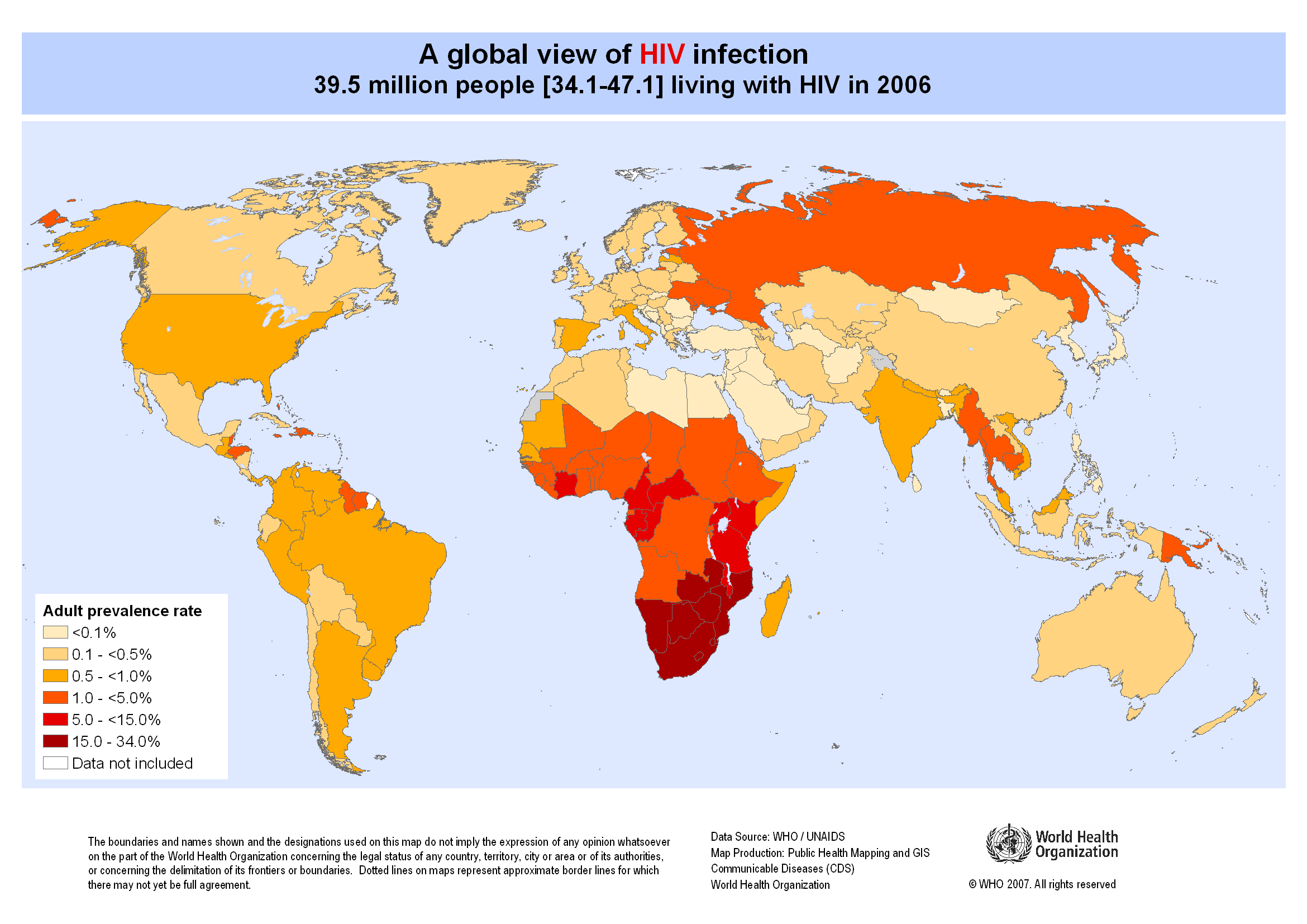
This map shows the global distribution of HIV burden. The concentration in Sub-Saharan Africa is striking — 67 percent of all people living with HIV are in this region. Nearly 40 million people worldwide are living with HIV as of 2023. Understanding the geographic distribution is essential for targeting engineering interventions like point-of-care diagnostics and water treatment in areas where HIV-positive individuals are immunocompromised and more vulnerable to waterborne disease.

HIV/AIDS

In 2023, 39.9 million people worldwide were living with HIV, of which 67% live in SSA

4.1 million people worldwide became newly infected
2.8 million people lost their lives to AIDS

New infections occur predominantly among the 15-24 age group.

First identified in the early 1980s. Has affected over 85 million people since the start of the epidemic.

Source: UNAIDS Global AIDS Update 2023

HIV Co-infections

Impact of TB on HIV

TB considerably shortens the survival of people with HIV/AIDS.
TB kills up to half of all AIDS patients worldwide.
TB bacteria accelerate the progress of AIDS infection in the patient

HIV and Malaria

Diseases of poverty
HIV infected adults are at risk of developing severe malaria
Acute malaria episodes temporarily increase HIV viral load
Adults with low CD4 count more susceptible to treatment failure

HIV/AIDS has affected over 85 million people since the start of the epidemic, with new infections concentrated in the 15-to-24 age group. A critical concept here is co-infections — TB kills up to half of all AIDS patients worldwide, and TB bacteria actually accelerate AIDS progression. HIV and malaria also interact: HIV-positive adults are more susceptible to severe malaria, and acute malaria episodes temporarily increase HIV viral load. These co-infection dynamics mean that addressing one disease in isolation is insufficient.

Non-Communicable Diseases (NCDs)

NCDs — chronic diseases not transmitted person-to-person — kill 41 million people each year (74% of all global deaths). 77% of NCD deaths occur in low- and middle-income countries, where health systems are least equipped to manage them.

NCDs with highest impact in low-income countries

Cardiovascular diseases — leading NCD killer globally (17.9M deaths/year); hypertension, rheumatic heart disease, and stroke are especially prevalent in SSA and South Asia
Chronic respiratory diseases (4.1M deaths/year) — driven by household air pollution from cooking with solid fuels (wood, charcoal, dung); 2.3 billion people still rely on polluting fuels, causing 3.2M premature deaths/year
Cancers (9.7M deaths/year) — cervical cancer (preventable via HPV vaccination) kills 350,000 women/year, 90% in LMICs; liver cancer linked to contaminated water and aflatoxin exposure
Diabetes (2.0M deaths/year) — type 2 diabetes rising fastest in LICs due to nutrition transition; 1 in 2 adults with diabetes are undiagnosed
Chronic kidney disease — strongly linked to contaminated drinking water (heavy metals, agrochemicals); CKD of unknown origin is epidemic in Central America, Sri Lanka, and parts of SSA

Environmental drivers in low-income settings

Air pollution — ambient + household air pollution causes 6.7M deaths/year; 9 out of 10 people breathe polluted air; LICs bear the highest burden per capita
Water quality — arsenic, fluoride, lead, and microbial contamination linked to cancers, kidney disease, skeletal fluorosis, and developmental harm in children; 2 billion people use contaminated water sources
Sickle cell disease — 300,000+ births/year (75% in SSA); 50–80% of affected children in Africa die before age 5 without treatment
Mental health — depression is the leading cause of disability in LMICs; treatment gap exceeds 90% in many low-income countries

Sources: WHO Global Status Report on NCDs 2024; WHO Household Air Pollution Fact Sheet 2024; Lancet Commission on Pollution and Health 2022

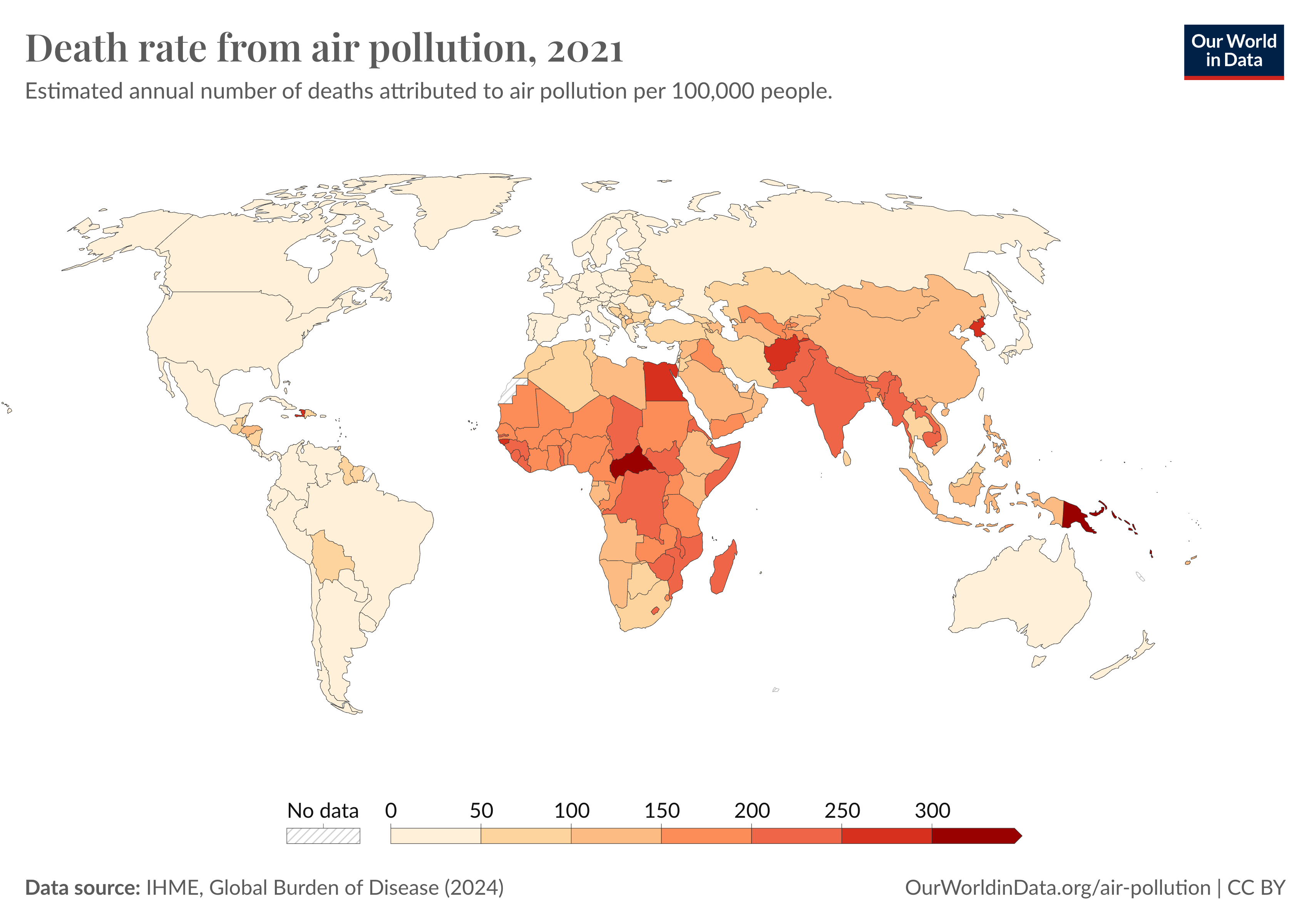
Non-communicable diseases are the other side of the coin. NCDs kill 41 million people per year — 74 percent of all global deaths — and 77 percent of NCD deaths occur in low- and middle-income countries. These are cardiovascular disease, chronic respiratory disease, cancers, and diabetes. For engineers, the key connection is environmental: household air pollution from cooking with solid fuels causes 3.2 million deaths per year, contaminated drinking water is linked to chronic kidney disease, and these are problems where engineering solutions exist.

Air Quality and Public Health

Air pollution is the single largest environmental health risk — responsible for 6.7 million premature deaths annually worldwide.

Two major exposure types

Ambient (outdoor) air pollution — 4.2M deaths/year; caused by vehicle emissions, industrial activity, power generation, and waste burning
Household air pollution — 3.2M deaths/year; caused by burning solid fuels (wood, charcoal, coal, dung) for cooking and heating. Affects 2.3 billion people, predominantly in LMICs

Health effects

Stroke and ischaemic heart disease (leading causes of air pollution deaths)
COPD and chronic respiratory disease
Lung cancer
Acute lower respiratory infections in children
Low birth weight, preterm birth, and impaired cognitive development

Key facts

9 out of 10 people breathe air exceeding WHO guideline limits
LMICs bear the heaviest burden — 89% of air pollution deaths
Children under 5 account for ~600,000 deaths from air pollution annually
Household air pollution disproportionately affects women and girls, who spend the most time near cooking fires

Source: WHO Air Pollution Fact Sheets 2024; Lancet Commission on Pollution and Health 2022

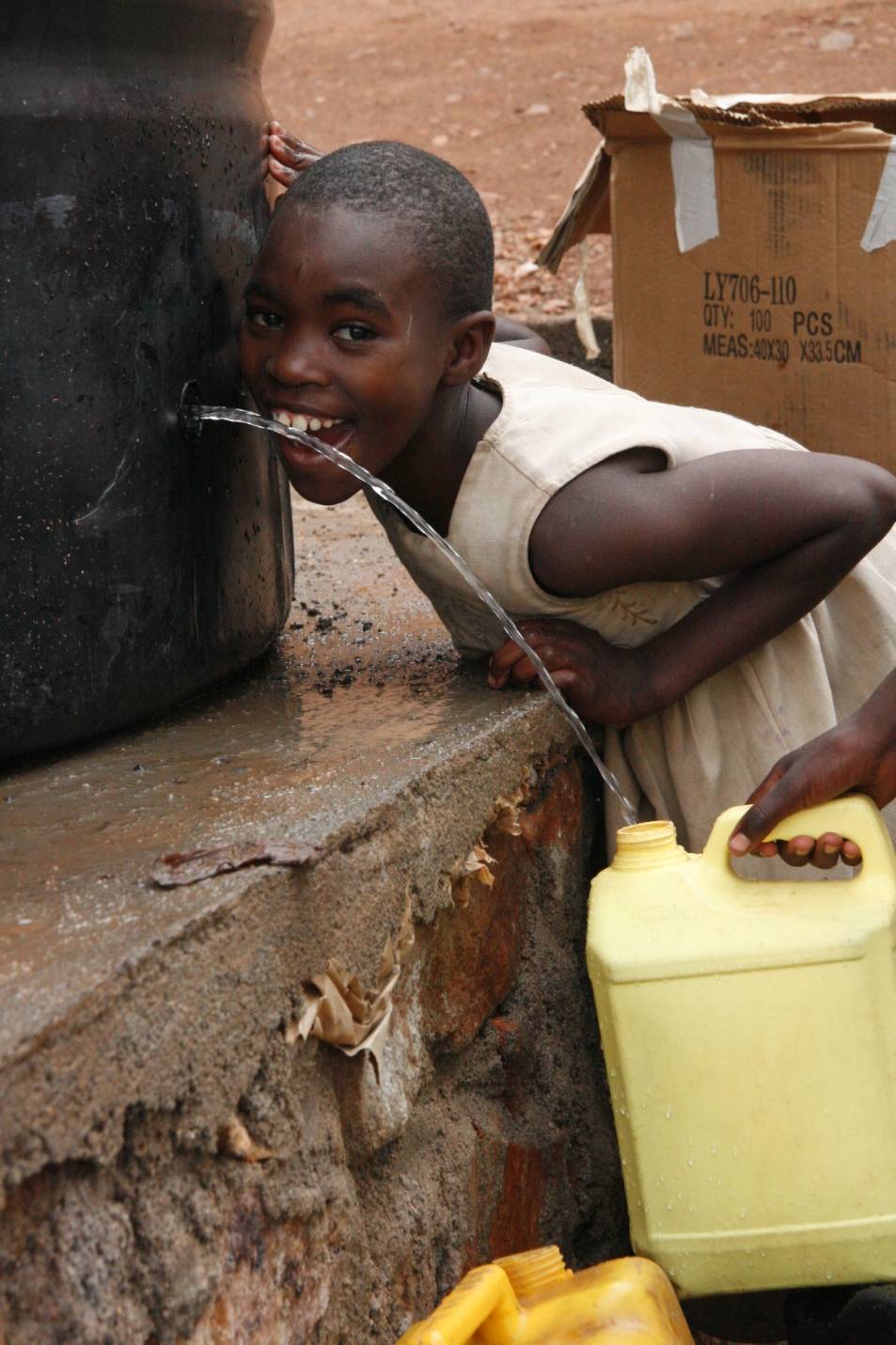
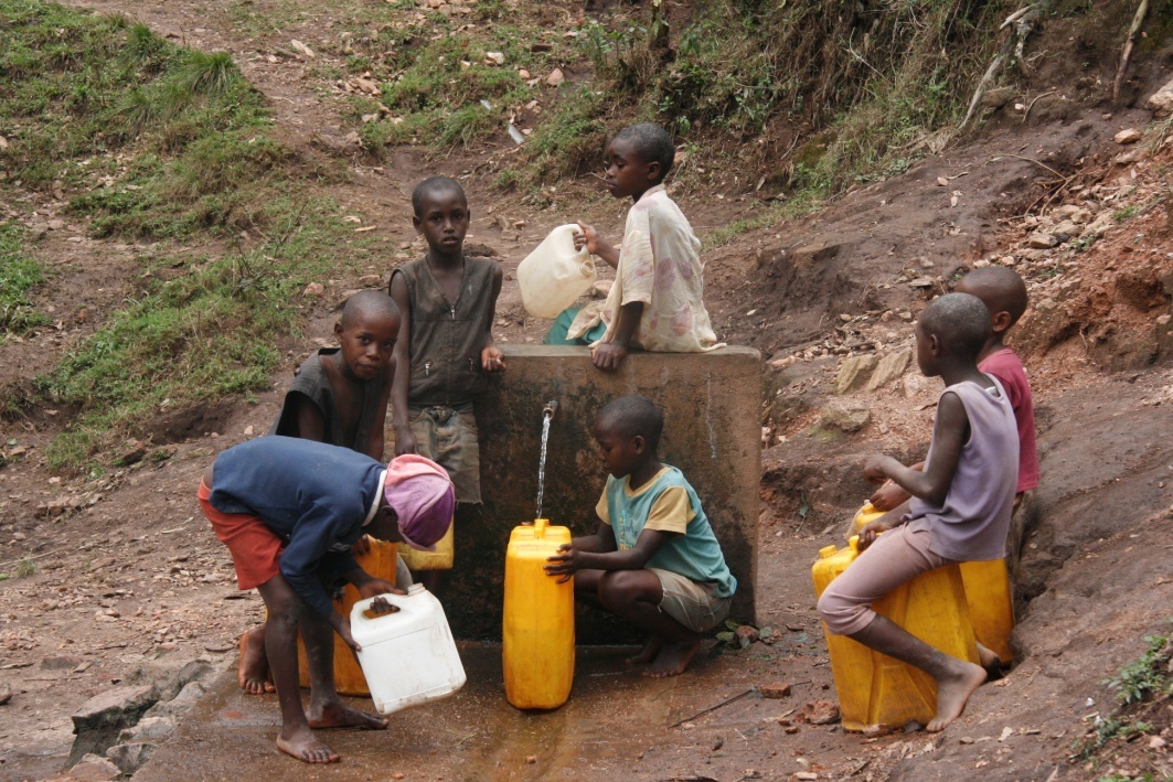
Air pollution is the single largest environmental health risk in the world — 6.7 million premature deaths annually. There are two major exposure types: ambient outdoor pollution from vehicles and industry at 4.2 million deaths, and household air pollution from cooking with solid fuels at 3.2 million deaths. Nine out of ten people breathe air exceeding WHO guidelines, and 89 percent of air pollution deaths are in low- and middle-income countries. This is a core area for engineering intervention — from clean cookstove design to air quality monitoring systems.

Water and Public Health

“No other single intervention in the history of medicine has saved as many lives and reduced as much suffering as the provisioning of uncontaminated water,” - Paul Edward

One billion people in the world lack access to clean drinking water

A leading cause of death worldwide
An estimated 1.4 million people die each year from inadequate water, sanitation and hygiene

Source: WHO, 2023

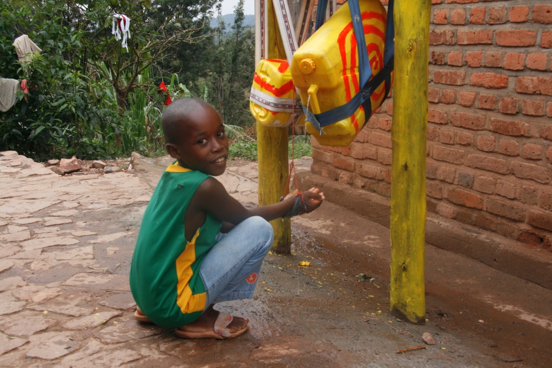
Water is perhaps the quintessential global health engineering challenge. The quote on this slide says it well — no other single intervention in the history of medicine has saved as many lives as the provisioning of uncontaminated water. One billion people still lack access to clean drinking water, and an estimated 1.4 million people die each year from inadequate water, sanitation, and hygiene. This is the domain where environmental engineers have the most direct and measurable impact on global health outcomes.

Sanitation and Public Health

Minimum Standards

Safe disposal excreta and sullage (greywater)

Avoid disposal within 15 meters of any water source

Provision of drainage
Disposal of waste
Control of insect and rodents

Sanitation is the other half of the WASH equation. The minimum standards are straightforward in principle — safe disposal of excreta away from water sources, provision of drainage, waste disposal, and vector control. But implementing these at scale in low-resource settings is an enormous engineering challenge. The images here show the reality of sanitation infrastructure in many parts of the world, and designing solutions that are affordable, maintainable, and culturally appropriate is where engineering expertise is essential.

Section

Epidemiology & Biostatistics

We're shifting gears now from the broader global health landscape into the methodological toolkit that underpins everything we've been discussing. Epidemiology and biostatistics are the quantitative backbone of public health, and as engineers, you'll find the logic here feels very familiar. We're going to learn how to measure disease, design studies, and interpret evidence.

John Snow & the Birth of Epidemiology

In 1854, a devastating cholera outbreak struck London’s Soho district, killing over 600 people. The prevailing “miasma theory” blamed foul air, but physician John Snow suspected contaminated water. Through meticulous mapping of deaths and interviews with residents, Snow traced the outbreak to a single source: the Broad Street pump.

The Broad Street pump memorial, Broadwick Street, London

Snow’s dot map — each bar marks a cholera death, clustered around the Broad Street pump

Snow convinced local authorities to remove the pump handle, and the outbreak subsided. His work established the foundations of epidemiology: systematic data collection, spatial analysis, and evidence-based public health intervention — decades before germ theory was accepted.

This is one of the greatest detective stories in the history of science. In 1854, John Snow didn't have germ theory, he didn't have a microscope powerful enough to see bacteria, but he had data and a map. By plotting cholera deaths and tracing water sources, he identified the Broad Street pump as the source of the outbreak. This is the founding moment of epidemiology, and it's fundamentally an engineering approach: observe, map, hypothesize, intervene.

Epidemiology — Defined

Adapted from: Last JM, ed. A dictionary of epidemiology. 2nd ed. Toronto, Canada: Oxford University Press; 1988.

Study of the distribution and determinants of health-related states among specified populations and the application of that study to the control of health problems

Purposes in Public Health Practice

Discover the agent, host, and environmental factors that affect health
Determine the relative importance of causes of illness, disability, and death
Identify those segments of the population that have the greatest risk from specific causes of ill health
Evaluate the effectiveness of health programs and services in improving population health

This is the formal definition of epidemiology, and I want you to notice how action-oriented it is. It's not just about studying disease for its own sake. The definition explicitly includes applying that knowledge to control health problems. As engineers, you're used to the idea that understanding a system is only useful if it leads to better design. Same principle here.

Epidemiology Key Terms

epidemic or outbreak: disease occurrence among a population that is in excess of what is expected in a given time and place.

cluster: group of cases in a specific time and place that might be more than expected.

endemic: disease or condition present among a population at all times.

pandemic: a disease or condition that spreads across regions.

rate: number of cases occurring during a specific period; always dependent on the size of the population during that period.

R₀ (basic reproduction number):

The average number of people one infected person will transmit the disease to in a fully susceptible population. R₀ > 1 means the epidemic grows; R₀ < 1 means it dies out. COVID-19 original strain R₀ ≈ 2.5; measles R₀ ≈ 15.

Let's get some vocabulary straight because these terms get misused constantly in the media. An epidemic is excess disease in a specific time and place. Endemic means the disease is always present at some baseline level. A pandemic crosses regions or goes global. And R0 is perhaps the most important number in infectious disease epidemiology. If R0 is greater than 1, each infected person infects more than one other person, and the epidemic grows exponentially. Measles with an R0 of 15 is incredibly contagious, which is why vaccination coverage needs to be so high.

Incidence vs. Prevalence

Incidence — the rate of new cases arising in a population over a defined time period.

Incidence rate = new cases ÷ population at risk ÷ time
Measures the risk of contracting a disease

Prevalence — the proportion of a population that has a condition at a specific point in time (or period).

Point prevalence = existing cases ÷ total population
Measures the burden of disease in a community

Example: Cholera in a Refugee Camp

Camp population: 10,000
100 new cases per week → incidence = 10 per 1,000 per week
Average illness lasts 5 days → ~71 active cases at any time → prevalence ≈ 0.7%

THE BATHTUB ANALOGY

🛁

Water flowing IN = new cases (incidence)

Drain = recovery or death

Water level = prevalence

High incidence + fast recovery = low prevalence
Low incidence + chronic disease = high prevalence

I love the bathtub analogy for this. Incidence is the water flowing in, prevalence is the water level, and recovery or death is the drain. A disease can have high incidence but low prevalence if people recover quickly, like a cold. Or low incidence but high prevalence if the disease is chronic, like diabetes. The cholera example makes this concrete: 100 new cases per week flowing in, but because each case resolves in about 5 days, the prevalence at any given moment is only about 71 active cases.

Measurement of Health Status

Life expectancy at birth — average years a newborn can expect to live given current mortality trends

Maternal mortality ratio — deaths from pregnancy-related complications per 100,000 live births

Infant mortality rate — deaths in infants under 1 year per 1,000 live births

Neonatal mortality rate — deaths under 28 days per 1,000 live births

Under-5 mortality rate — probability of dying before age 5, per 1,000 live births

GLOBAL COMPARISON

Metric	Norway	Sierra Leone
Life expectancy	83.3 yr	55.3 yr
Maternal mortality	2	443
Infant mortality	1.7	78.5
Under-5 mortality	2.4	105.6

Source: WHO Global Health Observatory, 2023

These are the metrics that define global health inequity in numbers. Look at the comparison between Norway and Sierra Leone. A child born in Sierra Leone is over 40 times more likely to die before age 5 than a child born in Norway. Maternal mortality is over 200 times higher. These aren't just statistics; they represent preventable deaths, and they're the reason this field exists. As engineers, when you see a 200-fold difference in a performance metric, that tells you the system is failing catastrophically in one context.

Understanding Dose-Response Curves

A dose-response curve describes the relationship between exposure to a substance (dose) and the resulting health effect (response).

Core Principles

Threshold vs. non-threshold — some agents have a safe level; others (radiation, some carcinogens) do not
Shape matters — linear, sigmoidal, supralinear, or U-shaped (hormesis)
Key metrics — ED₅₀ (effective dose for 50%), LD₅₀ (lethal dose for 50%), NOAEL (no observed adverse effect level)

Example: Paracetamol (Acetaminophen)

Therapeutic (500–1000 mg): pain relief
Overdose (>4 g/day): liver toxicity
Severe (>10 g): liver failure, death

The following slides apply dose-response thinking to water and air pollution.

SIGMOIDAL DOSE-RESPONSE CURVE

Paracetamol toxicity: sigmoidal curve from safe therapeutic range through liver damage threshold

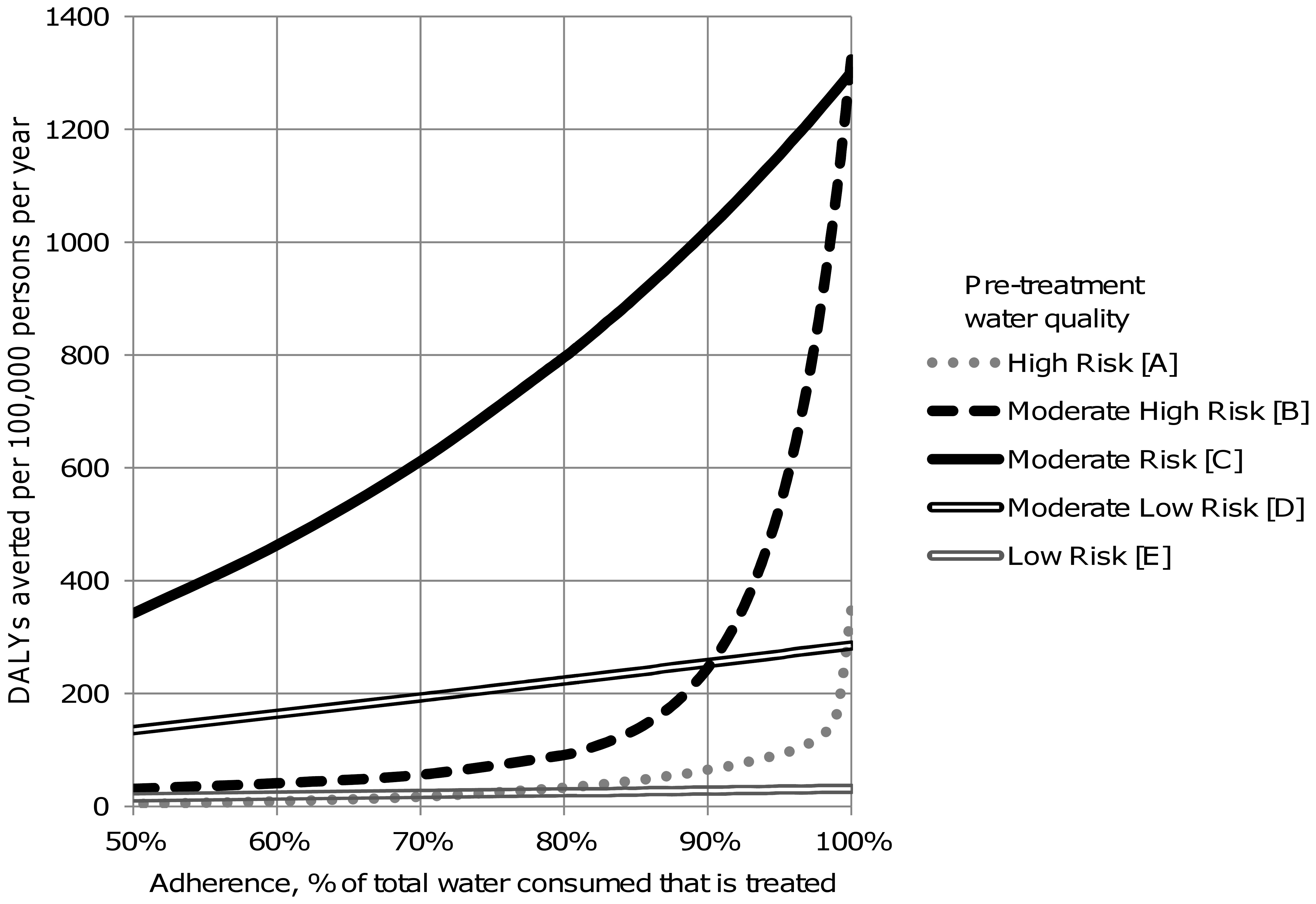
Dose-response is a concept you'll use constantly in environmental health engineering. The core idea is simple: the amount of exposure determines the magnitude of the effect. But the shape of that curve matters enormously for policy. Is there a safe threshold below which there's no effect? Is the curve linear or sigmoidal? The paracetamol example illustrates this beautifully. At therapeutic doses it relieves pain, but cross the threshold and the same molecule destroys your liver.

Dose-Response: Clean Drinking Water

The dose-response relationship for water quality interventions shows that health benefits increase with the level and consistency of adherence to clean water consumption.

Key observations

Even partial adoption of improved water sources reduces diarrhoeal disease risk by 30–40%
Consistent use of point-of-use treatment (filtration, chlorination) achieves the greatest reductions — up to 70–80% reduction in waterborne illness
Intermittent use provides limited protection; compliance is critical to achieving the full dose-response benefit
The curve is steepest at higher adherence levels — the last increment of compliance yields the largest marginal health gain

Source: Wolf et al., Cochrane Review on Water Quality Interventions, 2022

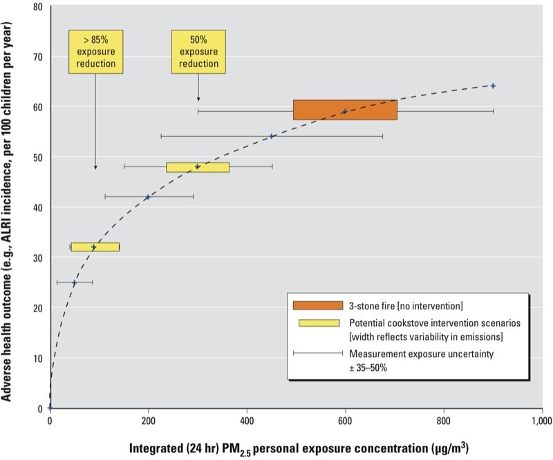
Adherence to clean drinking water dose-response curve

This slide applies dose-response thinking to one of the most important problems in global health: clean drinking water. Notice that the curve is steepest at higher adherence levels. That means the biggest health gains come from getting people from 80% compliance to 100%, not from 0% to 20%. This has huge implications for program design. It tells us that partial adoption provides some benefit, but consistent, sustained use is where the real health impact lies.

Dose-Response: Air Pollution Exposure

The dose-response curve for air pollution demonstrates a non-linear relationship between particulate matter (PM2.5) exposure and health outcomes, with the steepest risk at lower concentrations.

Key observations

The curve is supralinear — health risk per unit of PM2.5 is greatest at lower exposure levels, meaning even small reductions in already-low pollution yield significant benefits
At high exposure levels (common in LMICs), the curve flattens; large absolute reductions are needed to see proportional health improvement
Household air pollution from solid fuel cooking (PM2.5 often exceeds 500 µg/m³) sits on the flat portion — switching to clean fuels produces a dramatic shift along the curve
WHO guideline: annual mean PM2.5 < 5 µg/m³; 99% of the global population exceeds this threshold

Source: Global Burden of Disease Study 2021; Burnett et al., Integrated Exposure-Response Functions, 2014

Now look at how different the dose-response curve is for air pollution compared to water. This curve is supralinear, meaning the steepest part is at the low end. Small reductions in already-clean air produce the biggest health benefits per unit of pollution reduced. But here's the challenge for global health: most people in low-income countries are sitting way out on the flat part of the curve, exposed to PM2.5 levels 50 to 100 times the WHO guideline. That means you need dramatic reductions in exposure to see proportional health gains, which is exactly the challenge we'll see with cookstoves in Rwanda.

Modern Scenario: COVID-19 Outbreak Investigation

Timeline

Dec 2019: Cluster of pneumonia cases in Wuhan, China
Jan 7, 2020: Novel coronavirus identified (SARS-CoV-2)
Jan 20: Human-to-human transmission confirmed
Jan 30: WHO declares Public Health Emergency
Mar 11: WHO declares pandemic
Dec 2020: First vaccines authorized

Epidemiological Lessons

R₀ drove policy: original ~2.5, Delta ~5, Omicron ~10+ — recall that R₀ > 1 means exponential spread
Wastewater surveillance emerged as a key engineering tool
Genomic sequencing tracked variant evolution in real time
Disparities: LMICs received vaccines months to years later
7+ million confirmed deaths globally by 2024 (true toll estimated 15–25M)
mRNA vaccine platform: from sequence to authorized vaccine in 11 months

Apply your epi toolkit: This pandemic illustrates incidence (daily case curves), prevalence (active infections at peak), R₀ (transmission potential), and confounding (did lockdowns reduce spread, or did behavior change independently?).

COVID-19 was essentially a real-time epidemiology exam for the entire world. Every concept we've been discussing played out on a global stage. R0 drove lockdown policy. Incidence curves showed us exponential growth in real time. Confounding made it incredibly difficult to determine whether lockdowns themselves reduced spread or whether people changed behavior independently. And the engineering contributions were enormous: wastewater surveillance, rapid genomic sequencing, and the mRNA vaccine platform that went from viral sequence to authorized vaccine in 11 months.

Epidemiology Study Types

EXPERIMENTAL

Researcher assigns the exposure

Randomized Controlled Trial (RCT)
Gold standard — random assignment to treatment/control eliminates confounding. E.g., testing a new water filter vs. placebo.
Quasi-experimental
No random assignment. E.g., comparing villages that received a WASH program to those that did not.

OBSERVATIONAL

Researcher observes without intervening

Descriptive — who, where, when?

Case report / series — detailed account of one or a few patients
Cross-sectional survey — snapshot of a population at one point in time

Analytic — why? how?

Cohort study — follows exposed vs. unexposed forward in time → yields Risk Ratio
Case-control study — compares cases vs. controls backward → yields Odds Ratio

Understanding study types is critical because the type of study determines what conclusions you can draw. The RCT is the gold standard because randomization eliminates confounding. But RCTs aren't always possible or ethical. You can't randomly assign people to smoke. That's where observational studies come in. Cohort studies follow people forward in time and give you risk ratios. Case-control studies look backward from outcome to exposure and give you odds ratios. Each design has strengths and limitations, and as engineers designing health interventions, you need to know which evidence is strongest.

Confounding

A confounder is an extrinsic variable that is associated with both the exposure and the outcome, distorting the apparent relationship between them.

Exposure

Outcome

Confounder

Solid = true effect; Dashed = confounding paths

WASH Example

Exposure: Boiling drinking water

Outcome: Less diarrhoea

Confounder: Household wealth

Wealthier households are more likely to boil water and have better nutrition, sanitation, and healthcare — inflating the apparent benefit of boiling alone.

Methods to Control

Randomization (RCT)
Stratification by confounder
Matching cases & controls
Multivariate regression

Confounding is one of the most important concepts in all of epidemiology, and it's the main reason we need randomized trials. Look at the WASH example: wealthier households are more likely to boil their water AND more likely to have better nutrition and sanitation. So if you just observe that water-boilers have less diarrhea, you might be measuring the effect of wealth, not boiling. The methods to control for confounding, including randomization, stratification, matching, and regression, are tools you'll use in any research career.

Measuring the Association between Exposure and Outcome

The appropriate measure of association to use depends on the nature of the data

When exposure and outcome variables are dichotomous (two-level nominal data)

Odds ratio — use with case-control study (observational)
Risk ratio — use with cohort study (controlled)
Rate ratio — use with cohort study (controlled)

“Risk” refers to the probability of occurrence of an event or outcome.

“Odds” refers to the probability of occurrence of an event / probability of the event not occurring.

This slide introduces the key measures of association that connect exposure to outcome. The choice between odds ratio, risk ratio, and rate ratio isn't arbitrary. It depends on your study design. Case-control studies can only estimate odds ratios because you start by selecting cases and controls, so you don't know the true population risk. Cohort studies and RCTs can estimate risk ratios directly. The distinction between risk, which is a probability, and odds, which is the ratio of probability to its complement, is subtle but important.

Epidemiological Formulas

Rate Formula

To calculate a rate, we first need to determine the frequency of disease, which includes:

the number of cases of the illness or condition

the size of the population at risk

the period during which we are calculating the rate

RATE FORMULA

Rate = Cases ÷ Population at risk × 100

2 × 2 TABLE

	Disease +	Disease −
Exposed +	a	b
Exposed −	c	d

OR = (a×d) / (b×c) RR = [a/(a+b)] / [c/(c+d)]

Here's where the math comes in. The 2x2 table is the workhorse of epidemiology. You classify everyone by exposure status and disease status, then calculate your measure of association. The rate formula is straightforward: cases divided by population at risk over a time period. The odds ratio, ad over bc, and the relative risk, which compares the risk in exposed versus unexposed groups, are the two formulas you'll use most often. Get comfortable with these because we're about to work through an example.

Worked Example: Odds Ratio

The odds ratio (OR) quantifies the association between an exposure and an outcome in a case-control study.

Interpreting the OR:

OR = 1 — no association between exposure and outcome
OR > 1 — exposure is associated with higher odds of disease
OR < 1 — exposure is associated with lower odds (protective)

An OR of 2.97 means that smokers have approximately 3× the odds of developing lung cancer compared to non-smokers.

EXAMPLE: Smoking & Lung Cancer

	Cancer +	Cancer −
Smokers	688	650
Non-smokers	21	59

CALCULATION

OR = (688 × 59) / (650 × 21)

OR = 2.97

Smokers have ~3x the odds of lung cancer

Let's walk through this calculation together. We have a case-control study of smoking and lung cancer. Among the cancer cases, 688 were smokers and 21 were non-smokers. Among the controls without cancer, 650 were smokers and 59 were non-smokers. The odds ratio is 688 times 59 divided by 650 times 21, which equals 2.97. That means smokers had approximately three times the odds of developing lung cancer. This was the kind of evidence that eventually linked smoking to cancer, even before we understood the biological mechanism.

Sensitivity & Specificity

Sensitivity — the ability of a test to correctly identify those with the disease (true positive rate).

Sensitivity = a / (a + c) — “Of all sick people, how many test positive?”

Specificity — the ability of a test to correctly identify those without the disease (true negative rate).

Specificity = d / (b + d) — “Of all healthy people, how many test negative?”

Predictive Values

PPV = a / (a + b) — probability that a positive test is a true positive
NPV = d / (c + d) — probability that a negative test is a true negative
PPV depends heavily on prevalence: even a 99% specific test produces many false positives in low-prevalence settings

DIAGNOSTIC 2 × 2 TABLE

	Disease +	Disease −
Test +	a (TP)	b (FP)
Test −	c (FN)	d (TN)

TP = true positive, FP = false positive, FN = false negative, TN = true negative

Sensitivity and specificity are fundamental to understanding any diagnostic test, whether it's a rapid malaria test or a water quality sensor. A highly sensitive test rarely misses true cases but might flag some false positives. A highly specific test rarely gives false alarms but might miss some true cases. The key insight is about predictive value: even a 99% specific test will produce mostly false positives if the disease prevalence is very low. This is why mass screening in low-prevalence populations is problematic, and it's directly relevant to environmental monitoring where false alarm rates matter enormously.

Confidence Intervals, p-values & NNT

95% Confidence Interval

A range of values within which we are 95% confident the true population parameter lies.

For an OR or RR: if the 95% CI includes 1.0, the result is not statistically significant
Example: OR = 2.97 (95% CI: 1.83–4.82) — significant, because CI does not cross 1.0
Wider CI = less precision (smaller sample size); Narrower CI = more precision

p-value

The probability of observing a result this extreme (or more) if the null hypothesis were true.

Convention: p < 0.05 is considered “statistically significant”
A small p-value does not prove causation or clinical importance

Number Needed to Treat (NNT)

The number of patients who need to receive a treatment for one additional patient to benefit.

NNT = 1 / ARR

ARR = Absolute Risk Reduction = risk_control − risk_treatment

WASH Example:

Diarrhoea risk without filter: 25%
Diarrhoea risk with filter: 10%
ARR = 0.25 − 0.10 = 0.15
NNT = 1 / 0.15 ≈ 7
For every 7 households given a filter, 1 case of diarrhoea is prevented

NNT is especially useful for comparing the cost-effectiveness of global health interventions.

These three concepts tie together how we interpret study results. The confidence interval tells you the precision of your estimate. If it's wide, you need more data. If it crosses 1.0 for an odds ratio, the result isn't statistically significant. The p-value tells you how surprising the result would be if there were truly no effect, but remember that statistical significance doesn't mean clinical significance. And NNT is my favorite metric for communicating practical impact: for every 7 households you give a water filter, you prevent one case of diarrhea. That's the kind of number that helps policymakers make decisions.

Section

Public Health Interventions

Now that we have the epidemiological and statistical toolkit, let's talk about what we actually do with it. This section is about designing, implementing, and evaluating public health interventions. This is where engineering meets public health practice, where you move from understanding a problem to solving it.

Digital Epidemiology — Engineering Tools for Disease Surveillance

Wastewater Surveillance

Monitoring SARS-CoV-2, influenza, RSV, and poliovirus in sewage provides population-level disease tracking without individual testing. Over 70 countries now have wastewater surveillance programs.

Mobile & Satellite Data

Mobile phone mobility data tracked COVID-19 spread in real time. Satellite imagery monitors environmental risk factors: flooding, deforestation, urban heat islands, and vector breeding habitats.

Sensor Networks & IoT

Continuous water quality sensors (like the Lume TLF sensor), air quality monitors, and connected diagnostic devices enable real-time environmental health surveillance at scale.

This is where engineers are making some of the most exciting contributions to epidemiology right now. Wastewater surveillance was a game-changer during COVID because it gave us population-level disease data without requiring anyone to get tested. Mobile phone data and satellite imagery let us track disease spread and environmental risk factors at unprecedented scale. And sensor networks, including the kind of water quality sensors we develop at Virridy, enable real-time environmental health surveillance. This is the intersection of engineering and epidemiology.

Surveillance & Public Health Approach

Goal of Intervention

Develop strategies for particular groups to engage in change toward health

Provide a support system to initiate change and sustain positive behaviors

A Public Health Approach

Surveillance → Risk Factor Identification → Intervention → Implementation → Evaluation

Surveillance

What is the problem?

→

Risk Factor ID

What is the cause?

→

Intervention

What works?

→

Implementation

How do you do it?

→

Evaluation

Did it work?

This framework shows the public health approach as a cycle. You start with surveillance to understand the problem, then identify risk factors, then design and implement an intervention, and finally evaluate whether it worked. That evaluation feeds back into surveillance, and the cycle continues. Notice that this is essentially the engineering design cycle applied to health. The key point is that interventions need to both initiate behavior change and sustain it over time, which turns out to be the hardest part.

Approaches to Interventions

Personal responsibility and action

Utilitarian Approaches – "Greatest good for the greatest number"

Including non Health Systems Interventions.

Regulations and Laws

Partnerships and Collaboration

Enlightened Self Interest

Education

Develop favorable attitudes towards the behavior

Training (i.e. Community health workers)

Participatory engagement

Provide sustainable access

Utilizing underlying skills of the local people

Supportive Environment

Utilizing families, local organizations, community leaders, policy makers

There are many different levers for changing health behavior. Personal responsibility approaches put the onus on individuals, but that has limits when people face structural barriers. Utilitarian approaches target the greatest good for the greatest number. Regulations can be powerful, like seatbelt laws or fluoridation. But in global health, education and community engagement are often the primary tools. Training community health workers, using participatory methods, and working through local leaders and families creates a supportive environment for sustainable change.

Behavior Change

Why Do People NOT Change Behavior?

Do they understand the message?

Do they see themselves as vulnerable?

Do they trust the ones who present the message?

Do they think the benefits of change are worth the long-term benefits?

Is it too costly?

Does change contradict with their religious beliefs?

Health Belief Model

Perceived susceptibility – risk of acquiring the disease

Perceived severity – perception on the risk of acquiring the disease

Perceived benefits – is it worth the change?

Perceived barriers – obstacles to achieving health change

Cue to action – what will trigger this change?

Self-efficacy – how confident is the person to successfully perform a behavioral change?

This is one of the most humbling topics in public health. We can develop a technology that works perfectly in the lab, but if people don't use it consistently, it doesn't matter. The Health Belief Model explains why: people weigh their perceived susceptibility, the perceived severity of the disease, the perceived benefits and barriers of the intervention, and their own self-efficacy. If a mother doesn't believe her child is at risk from untreated water, or if the filter is inconvenient, she won't use it. Understanding these barriers is as important as the engineering design itself.

Randomized Controlled Trial (RCT)

Efficacy vs. Effectiveness

Efficacy — Does the intervention work under ideal, controlled conditions? Participants are closely monitored, protocols are strictly followed, and non-compliant subjects may be excluded. Answers: "Can it work?"

Effectiveness — Does the intervention work under real-world conditions? Studies include typical populations, variable adherence, and routine delivery systems. Answers: "Does it work in practice?"

An intervention can show high efficacy but low effectiveness if uptake, adherence, or delivery is poor at scale — a common gap in global health programs.

Study Population

↓ Randomization

Treatment Group

Receives intervention

Control Group

No intervention / placebo

↓ Follow-up ↓ Follow-up

Compare Outcomes

The RCT is the gold standard for evaluating interventions, and I want to emphasize the critical distinction between efficacy and effectiveness. Efficacy asks whether an intervention can work under ideal conditions, with perfect adherence and close monitoring. Effectiveness asks whether it works in the real world, with all the messiness of actual human behavior. An intervention can have high efficacy but low effectiveness if people don't adopt it or use it correctly. This gap between efficacy and effectiveness is the central challenge of global health engineering, and it's exactly what we saw in Rwanda.

Cost-Effectiveness Analysis

With limited resources, decision-makers must prioritise interventions that produce the greatest health gain per dollar spent.

Key Concepts

DALY (Disability-Adjusted Life Year) = YLL + YLD — one DALY = one lost year of healthy life
ICER = ΔCost / ΔDALYs averted — the incremental cost per unit of health gained
Willingness-to-pay threshold — WHO suggests 1–3× GDP per capita per DALY averted

Decision Rules

ICER < GDP/capita → highly cost-effective
ICER 1–3× GDP/capita → cost-effective
ICER > 3× GDP/capita → not cost-effective

WASH Intervention Comparison

Intervention	$/DALY averted
Oral rehydration salts	$50–100
Point-of-use chlorination	$100–300
Household water filters	$300–800
Piped water to premises	$1,000–5,000

Estimates vary by context. Source: DCP3, WHO-CHOICE

When you have limited resources, which is always the case in global health, you need a systematic way to compare interventions. The DALY, or disability-adjusted life year, gives us a common currency for measuring health outcomes. One DALY equals one lost year of healthy life. The ICER tells you the incremental cost per DALY averted. Look at the WASH comparison table: oral rehydration salts cost 50 to 100 dollars per DALY averted, while piped water costs 1,000 to 5,000. That doesn't mean piped water is bad, but it tells you where each dollar has the greatest impact.

Implementation Science

The study of methods to promote the adoption, fidelity, and sustainability of evidence-based interventions in real-world settings.

Adoption

Will the target population take up the intervention?

Cultural acceptability
Perceived benefit vs. cost
Community champions & peer effects

Fidelity

Is it used correctly and consistently?

Training quality & supervision
Self-report vs. sensor gap (67% vs. 37%)
Stove stacking — partial adoption

Sustainability

Will effects persist after external support ends?

Funding model (carbon credits vs. aid)
Local capacity & supply chains
Government ownership

The gap between efficacy and effectiveness is almost always an implementation problem. The Rwanda case study illustrates all three challenges.

Implementation science is the field that specifically studies the gap between what works in trials and what works in practice. It focuses on three pillars: adoption, fidelity, and sustainability. Will people take up the intervention? Will they use it correctly? And will the effects persist after the research team leaves? Notice the self-report versus sensor gap: 67% versus 37%. That's a massive discrepancy, and it tells us that without objective monitoring, we systematically overestimate how well our interventions are performing. The Rwanda case study we're about to see illustrates every one of these challenges.

Health System Strengthening

Effective interventions require functioning health systems. The WHO framework identifies six building blocks essential to health system performance.

Service Delivery

Accessible, safe, quality health services that meet population needs

Health Workforce

Sufficient, skilled, motivated workers — Rwanda: 45,000 CHWs are the backbone

Health Information

Surveillance, vital registration, HMIS — data for decision-making

Medical Products

Medicines, vaccines, diagnostics — equitable access & supply chain

Financing

Adequate funding, risk pooling, universal health coverage goals

Leadership & Governance

Strategic policy, regulation, accountability, anti-corruption

Engineering contribution: Engineers build the infrastructure, information systems, supply chains, and monitoring tools that make health systems function. WASH infrastructure is a core building block.

Even the best intervention will fail without a functioning health system to deliver it. The WHO identifies six building blocks, and I want you to think about where engineering fits into each one. Engineers build the infrastructure for service delivery, design the information systems for health data, manage the supply chains for medical products, and develop the monitoring tools that support governance and accountability. In Rwanda, the community health worker system with 45,000 CHWs is the backbone of the health system, and it's what made our intervention possible.

Case Study

Rwanda Tubeho Neza
Water Filter & Cookstove Programme

Everything we've been talking about in epidemiology, study design, implementation science, and behavior change comes together in this case study. Tubeho Neza means 'Live Well' in Kinyarwanda. This was a large-scale, cluster-randomized controlled trial that my team led in western Rwanda, distributing water filters and improved cookstoves to over 100,000 households. It's a story of both success and humbling lessons about what happens when interventions meet real-world conditions.

Rwanda — Country Context

Key Indicators

Population: 14 million (2024)
GDP per capita: ~$800
Under-5 mortality: 38 per 1,000 live births
Over 80% rely on firewood as primary fuel
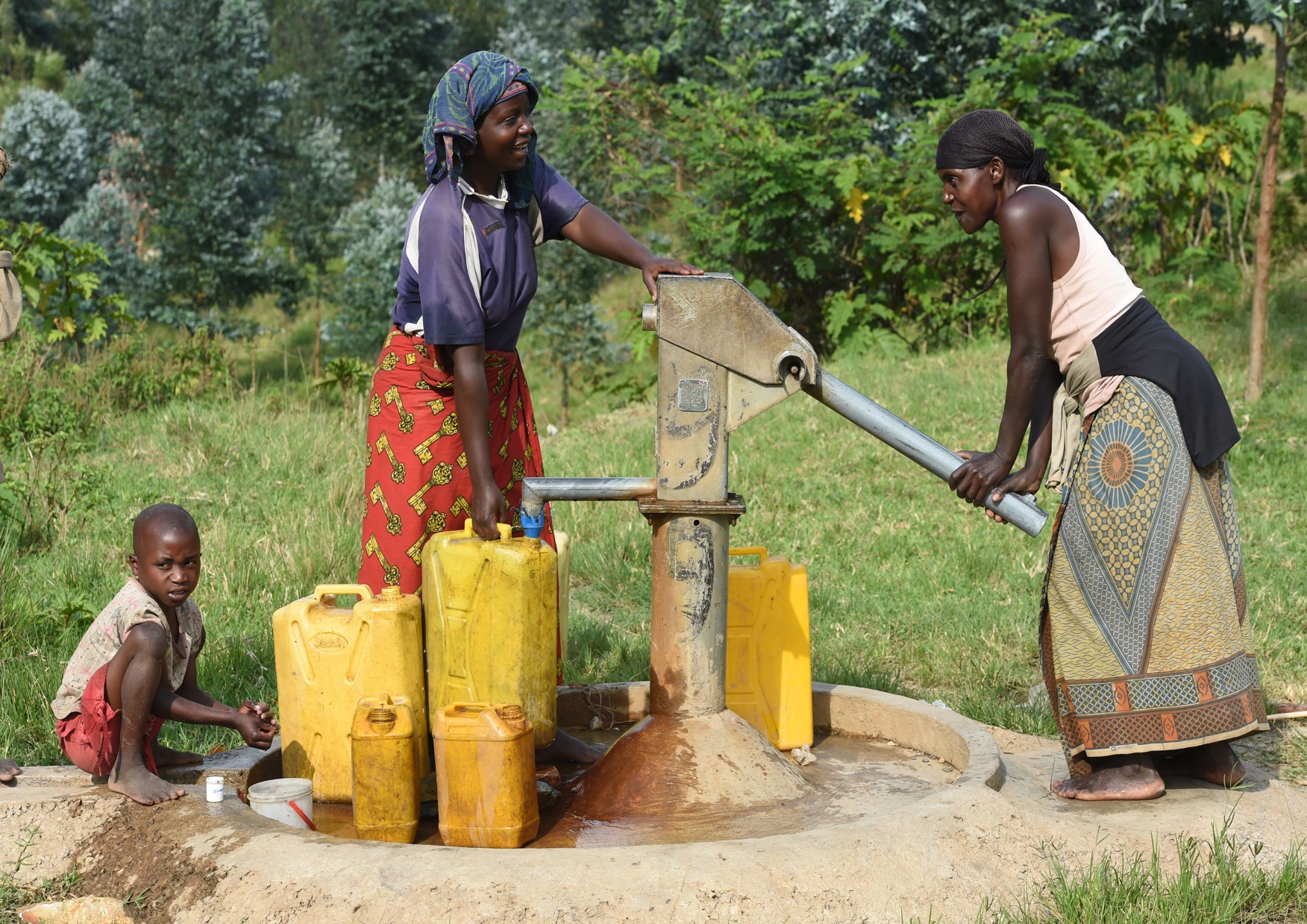
Most rural households drink untreated water

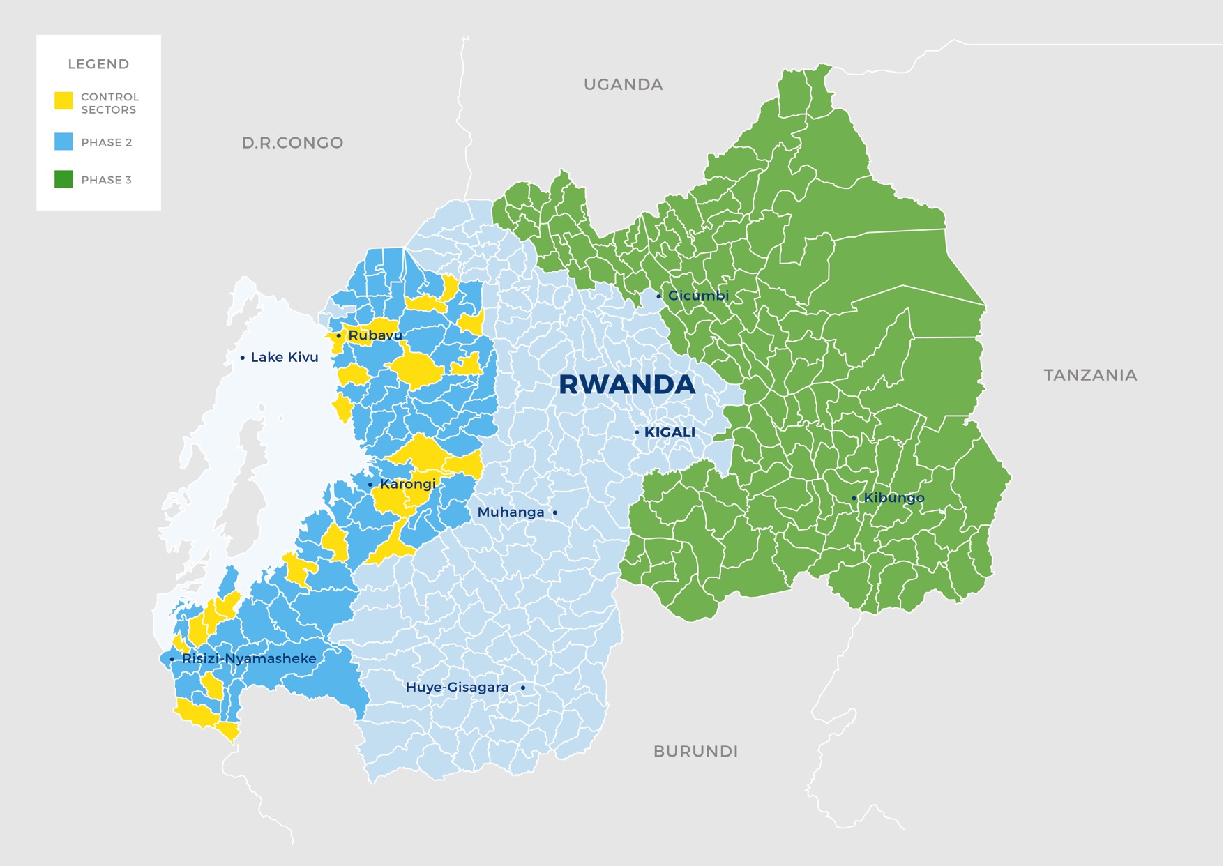
Study Location

Western Province, Rwanda — 96 sectors cluster-randomized, reaching 101,000 households with water filters and improved cookstoves.

Let me set the scene. Rwanda is a small, densely populated country in East Africa with about 14 million people and a GDP per capita of roughly 800 dollars. Over 80% of the population relies on firewood for cooking, and most rural households drink untreated surface water. Under-5 mortality is 38 per 1,000 live births, which is dramatically better than it was 20 years ago but still 15 times higher than Norway. Our study was based in Western Province, where we cluster-randomized 96 sectors to reach 101,000 households.

Programme Implementation

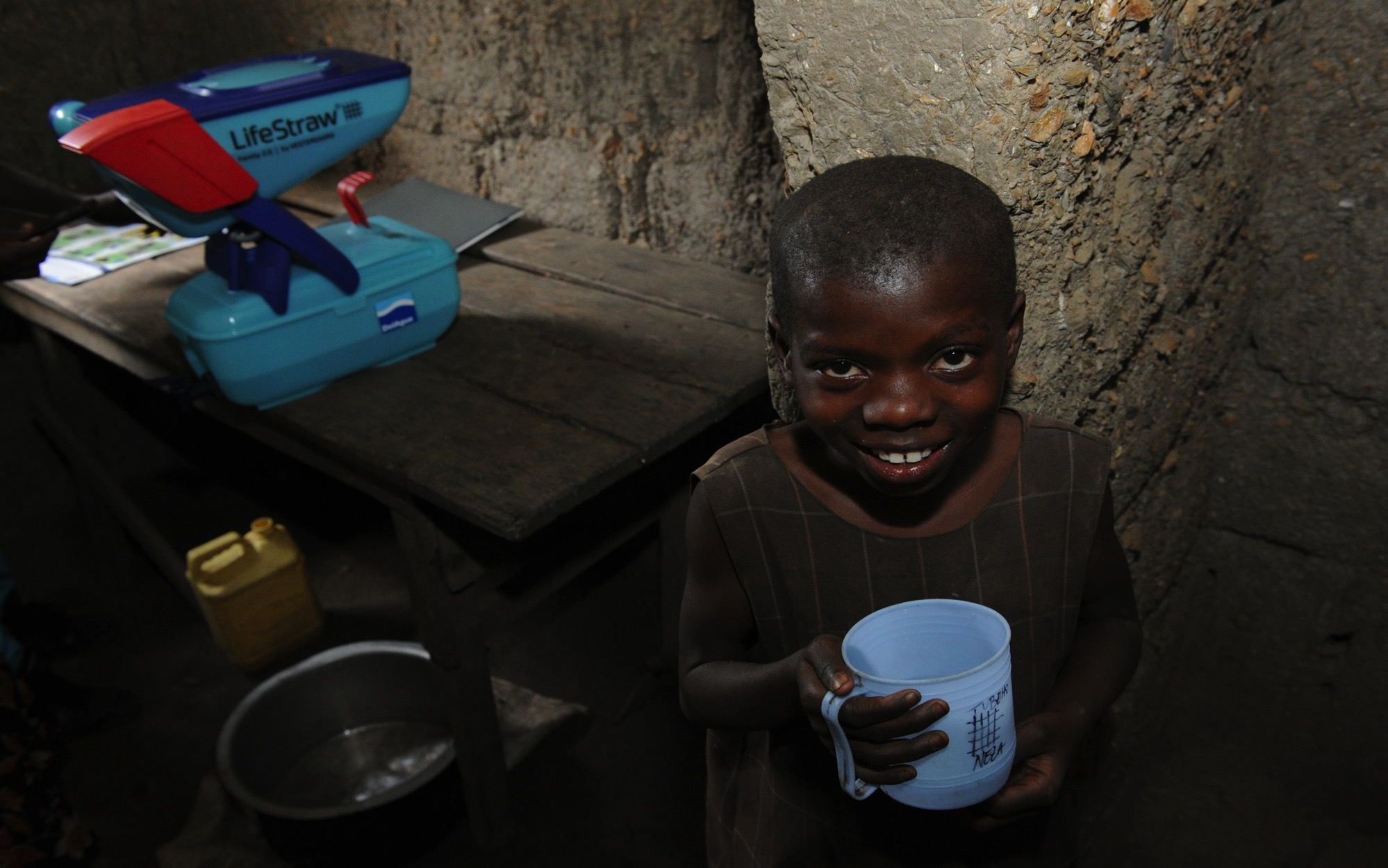
LifeStraw Family 2.0 water filter in household

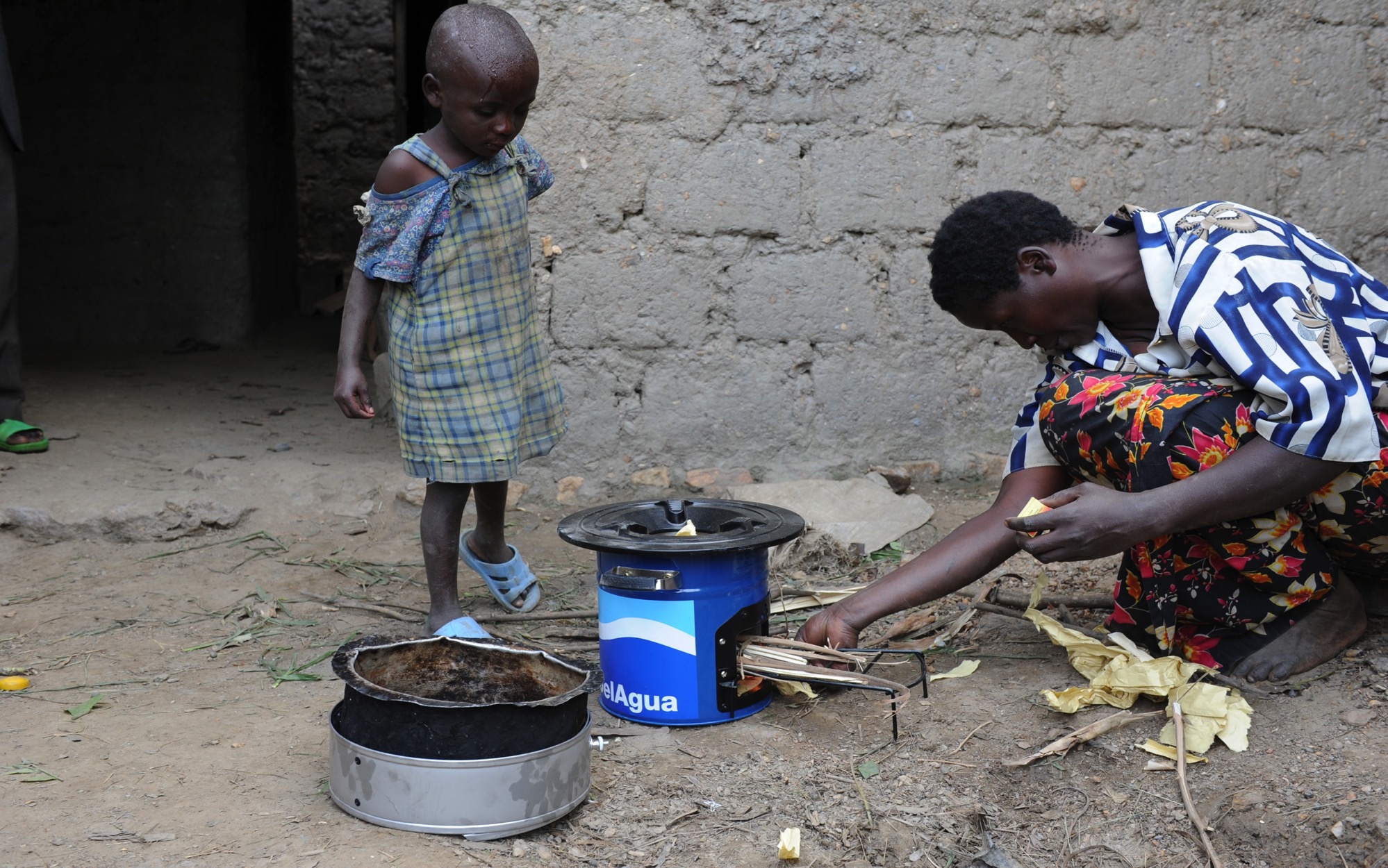
EcoZoom Dura improved cookstove in use

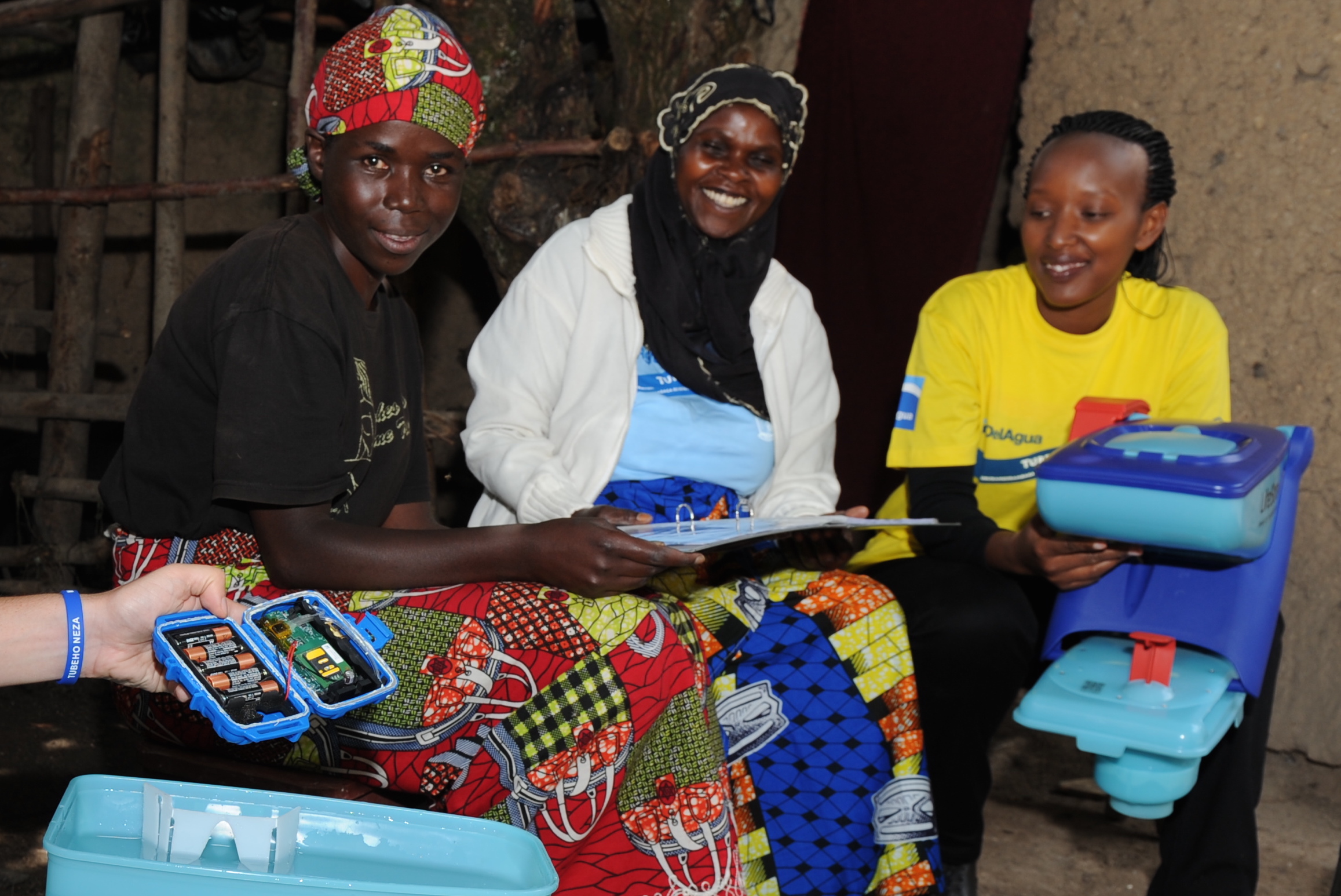
Electronic sensor monitoring deployment

Here you can see the three main components of the programme. On the left, the LifeStraw Family 2.0 water filter, which is a gravity-fed hollow fiber membrane filter that removes bacteria and parasites. In the middle, the EcoZoom Dura improved cookstove, designed to burn wood more efficiently and reduce smoke. And on the right, the electronic sensors we deployed to objectively monitor whether people were actually using these technologies. That third component turned out to be the most important contribution.

Community health worker training in Rwanda

This is a community health worker training session in Rwanda. These CHWs were the human infrastructure of our programme. They distributed the filters and stoves, conducted household visits, and provided ongoing education and support. Rwanda's CHW system is one of the strongest in sub-Saharan Africa, with 45,000 volunteers covering every village in the country. Without them, reaching 101,000 households would have been impossible.

Key Results — Tubeho Neza Trial

Health Outcomes (Children Under 5)

29% reduction in 7-day prevalence of diarrhea
25% reduction in acute respiratory infections
97.5% reduction in fecal contamination of drinking water
38% reduction in cryptosporidium seroconversion

Air Quality — A Cautionary Finding

Personal PM2.5 exposure remained unchanged despite improved cookstoves
Stove stacking: traditional fire use increased from 24% to 49% over study period

The Adherence Problem

Self-reported filter use: 67%
Sensor-detected filter use: 37%
Self-reported stove use: 84%
Sensor-detected stove use: 37%
Reported use declined: 75% → 68% → 65% across survey rounds

Economics

5-year programme cost: ~$12 million
Estimated 5-year benefit: >$66 million
Fuelwood savings: 65,000 tons — enough to reverse regional deforestation

Sources: Kirby, Nagel et al. (2019) PLoS Medicine; Thomas et al. (2018) Lancet Planetary Health; Thomas (2019) The Conversation

Here are the headline results, and they tell a nuanced story. On the water side, we saw a 97.5% reduction in fecal contamination and a 29% reduction in childhood diarrhea. Those are strong results. But on the air quality side, personal PM2.5 exposure was unchanged despite the improved cookstoves, because of stove stacking. Households kept using their traditional fires alongside the new stoves. And the adherence data is perhaps the most important finding: self-reported filter use was 67%, but sensor-detected use was only 37%. People were telling us they were using the filter almost twice as much as they actually were. This gap fundamentally changed how I think about intervention evaluation.

Technology & Digital Monitoring

Water Filters

LifeStraw Family 2.0 household water filters
Significant microbiological effectiveness reducing E. coli contamination
Free distribution with carbon waiver for credit generation

Remote Sensing Innovation

Electronic sensors remotely transmitting usage data
Sensor-reported use was substantially lower than self-reported use
Demonstrated critical value of objective digital monitoring
Published in ACS Environmental Science & Technology

Carbon Credit Model

Pay-for-performance model funded by voluntary carbon credits
Health, livelihood, and environmental benefits substantially outweighed costs
Fuel savings and averted healthcare costs = largest economic gains

The technology and monitoring story is really the engineering contribution of this project. The LifeStraw filters were highly effective at removing pathogens when used, which is the efficacy story. But the sensor data revealed a very different effectiveness story. We published these findings in ACS Environmental Science and Technology, and they demonstrated that self-reported data systematically overestimates use. The carbon credit model was also innovative because it created a pay-for-performance financing mechanism. Health and economic benefits substantially outweighed costs, with fuel savings and averted healthcare being the largest gains.

Scale, Carbon Finance & Lessons Learned

Scale

101,000 households received filters + cookstoves (2014)
250,000 additional cookstoves distributed (2015) reaching ~1 million more people
First-ever UN CDM and Gold Standard programmes earning carbon credits for water treatment

Carbon Credit Financing Model

Carbon credit revenue funded distribution, training, and monitoring
Did not rely on traditional aid/USAID funding — prescient given the 2025 USAID shutdown
Now expanded via Virridy Carbon to Rwanda, Burundi, DRC, Madagascar, Kenya, Tanzania

Key Lessons

Self-report ≠ reality — sensor data revealed ~2x overestimation of use
Adherence declines — sustained engagement requires ongoing CHW visits
Stove stacking — households used both improved and traditional stoves, limiting air quality gains
Water treatment worked, cookstoves didn't — 97.5% water quality improvement vs no PM2.5 change
Integration matters — combining with Rwanda's existing CBEHPP infrastructure improved reach
Alternative financing — carbon credits provide sustainable revenue independent of aid budgets

Let me highlight the key takeaways from this entire programme. First, scale: we reached 101,000 households initially and then distributed 250,000 additional cookstoves. These were the first-ever carbon credit programmes for water treatment under both the UN CDM and Gold Standard. Second, the lessons: self-report does not equal reality, adherence declines over time without sustained engagement, stove stacking limited air quality gains, but water treatment genuinely worked. And third, the financing model: carbon credits provided sustainable revenue independent of traditional aid budgets. Given the 2025 USAID shutdown, that independence turned out to be prescient.

Published Research (13 Papers)

Title	Journal	Link
Health, livelihood, and environmental impacts of the Tubeho Neza programme	The Lancet Planetary Health	Open
Effects of adding household water filters to Rwanda's CBEHPP	Nature — npj Clean Water	Open
Assessing Impact of Water Filters and Cookstoves: A Randomised Controlled Trial	PLOS ONE	Open
Designing and Piloting a Program to Provide Water Filters and Cookstoves	PLOS ONE	Open
Cost-benefit analysis of livelihood, environmental and health benefits	ScienceDirect	Open
Use, microbiological effectiveness and health impact of a household water filter	ScienceDirect	Open
Study design of a cluster-randomized controlled trial	ScienceDirect	Open
Process evaluation and assessment of use	BMC Public Health	Open
Use of Remotely Reporting Electronic Sensors	ACS Env. Sci. & Tech.	Open
Integration of Household Water Filters with Community-Based Sanitation	MDPI Sustainability	Open
Geospatial-temporal, demographic, and programmatic adoption characteristics	Cogent Engineering	Open
Assessing use, exposure, and health impacts (Dissertation)	Semantic Scholar	Open
Lessons from Rwanda on tackling unsafe drinking water and air pollution	The Conversation	Open

This body of work generated 13 peer-reviewed publications across top journals including The Lancet Planetary Health, Nature, PLOS Medicine, and ACS Environmental Science and Technology. I'm showing you this not to list papers but to make a point: rigorous research on real-world implementation challenges is publishable and impactful. These papers have shaped how the field thinks about adherence monitoring, the efficacy-effectiveness gap, and carbon finance for health interventions. The research continues through Virridy Carbon, which has now expanded this model across six countries in East Africa.

From Research to Methodology

The Tubeho Neza trial is used throughout the next section as a detailed case study for understanding research methodology — from study design and bias to statistical analysis and causal inference.

Study Design

Cluster RCT, 96 sectors, 3:1 randomization

Measurement

Self-report vs sensors, information bias

Analysis

GEE regression, clustering, missing data

Causal Inference

Counterfactuals, confounding, ITT analysis

We've just walked through the Rwanda case study in detail — the intervention design, the results, the complications. Now I want to use that same study as a running example to teach you research methodology. Every concept we cover next — bias, study design, statistics, causal inference — I'll illustrate with specific data from Tubeho Neza so you can see how these abstract ideas play out in a real trial.

Section

Research Methodology

Methodological Considerations in Evaluating Global Health Interventions

This section is really the methodological core of the course. We're going to cover the key concepts you need to critically evaluate any global health study — how to spot bias, understand study design trade-offs, and interpret statistical results. I'll keep coming back to the Rwanda trial as our working example throughout.

Applying Methodology to Tubeho Neza

We now use the Rwanda water filter & cookstove trial (covered in the previous section) as a running case study for research methodology.

The core evaluation questions that will drive this section:

Did this program actually reduce diarrhea in children under 5? Acute respiratory infections?
Did it improve household water quality? Personal air quality (PM_2.5)?
How do we know the measured effects are real and not artefacts of bias?

Each topic below will reference specific Rwanda data to illustrate the methodology in action.

Published: Kirby, Nagel et al. (2019) PLoS Medicine | Design: Nagel, Kirby et al. (2016) CCTC

Here are the questions we're going to systematically work through. Did this program actually reduce childhood diarrhea and respiratory infections? Did it improve water quality and air quality? And critically, how do we know the effects we measured are real and not just artifacts of how the study was designed or how we collected data? These are the questions that separate rigorous evidence from wishful thinking.

Biased Approaches to Evaluation

Biased Approach #1: Before vs. After

Diarrhea prevalence drops from 15% before distribution to 9% after. Tempting conclusion: a 40% reduction.

Seasonality: The rainy season ended between measurements — diarrhea is seasonal
Concurrent changes: Rotavirus vaccine campaigns, economic growth, other WASH programs
Regression to mean: Starting during a disease spike means prevalence naturally returns to average

Before/after comparisons confound the intervention effect with all temporal changes.

Biased Approach #2: Users vs. Non-Users

Filter users have 40% less diarrhea — but users are more educated, practice handwashing, have better healthcare access.

This is selection bias: the comparison group is not exchangeable with the treatment group.

Rwanda Trial: Baseline diarrhea was 15.3% (intervention) vs 13.7% (control) — already different before intervention.

These are the two most common mistakes I see in program evaluation. The first is before-and-after comparisons — diarrhea went down after we distributed filters, so the filters must have worked. But what else changed? The rainy season ended, a vaccine campaign launched, the economy grew. The second mistake is comparing users to non-users — people who choose to use the filter are systematically different from those who don't. This is why we need rigorous study designs.

The Three Systematic Threats to Validity

We introduced confounding in the Epidemiology section. Here we add selection bias and information bias — the complete triad of systematic error.

Every epidemiological study faces two kinds of error. Random error shrinks with larger samples. Systematic error — bias — does not.

C — Confounding

A third variable distorts the exposure-outcome relationship because it is associated with both.

e.g., Wealthier households use filters AND have less diarrhea

S — Selection Bias

The study sample is not representative, or loss to follow-up differs systematically between groups.

e.g., Analyzing only clinic visitors misses healthy children

I — Information Bias

Systematic errors in how exposure, outcome, or covariates are measured.

e.g., Caregivers over-report filter use (social desirability)

These are the three big enemies of valid research — confounding, selection bias, and information bias. I want you to memorize this triad because every time you read a study, you should be asking: could confounding explain this result? Is there selection bias in who was studied? Is there information bias in how outcomes were measured? Random error shrinks with bigger samples, but these systematic errors do not — they require careful design to address.

Confounding, Selection Bias & Information Bias

Confounding: When a Third Variable Creates a False Association

Three criteria for a confounder: (1) associated with the exposure, (2) independently associated with the outcome, (3) not on the causal pathway.

Control methods: Design: randomization, restriction, matching. Analysis: stratification, regression, propensity scores.

Selection Bias: When Who Gets Studied Distorts Findings

Loss to follow-up: Differential attrition biases the comparison
Collider bias: Conditioning on a common effect creates spurious associations
Volunteer/self-selection: Study volunteers differ systematically from non-volunteers

Information Bias: When Measurement Is Systematically Wrong

Differential misclassification: Error differs between groups (recall bias, courtesy bias)
Non-differential misclassification: Equal error across groups — biases toward the null

Now let's dig deeper into each type. For confounding, remember the three criteria — the confounder must be associated with both the exposure and the outcome, and it can't be on the causal pathway. Look at those numbers at the bottom: 67% self-reported filter use versus 37% sensor-detected use. That's information bias in action — a nearly two-fold overestimation. And it was even worse for stoves. This is why we deployed sensors alongside surveys in this trial.

Recognizing Bias & Direction of Effects

Stage	Critical Question	Bias Addressed
Design	Is treatment assignment independent of confounders?	Confounding
Design	Can participants be blinded to assignment?	Information
Enrollment	Is the sample representative of the target population?	Selection
Follow-Up	Is attrition differential between groups?	Selection
Measurement	Are outcomes assessed identically in all groups?	Information
Analysis	Have confounders been identified via DAG and adjusted?	Confounding

Direction of Bias

Non-differential misclassification: Toward null — dilutes the true effect
Uncontrolled confounding: Either direction — depends on the confounder
Differential misclassification: Either direction — unpredictable (recall bias, courtesy bias)

This table is a practical checklist you can use when reviewing any study. At every stage — design, enrollment, follow-up, measurement, analysis — there's a critical question to ask. I also want you to understand the direction of bias. Non-differential misclassification biases toward the null, meaning it makes you underestimate the true effect. That's important because it means if you still find a significant result despite measurement noise, the true effect is probably even larger.

Study Design Hierarchy for Causal Inference

Each step down the hierarchy requires stronger assumptions to claim causation.

Randomized Controlled Trial (RCT)

Randomization creates exchangeable groups. Gold standard for causal inference.

Quasi-Experimental Designs

Exploit natural variation (DiD, RDD, ITS). No random assignment but clever design.

Cohort Study

Follow exposed/unexposed over time. Temporal ordering established.

Case-Control Study

Identify cases, select controls, look back. Efficient for rare outcomes.

Cross-sectional study: Snapshot — exposure and outcome measured simultaneously. Weakest for causation.

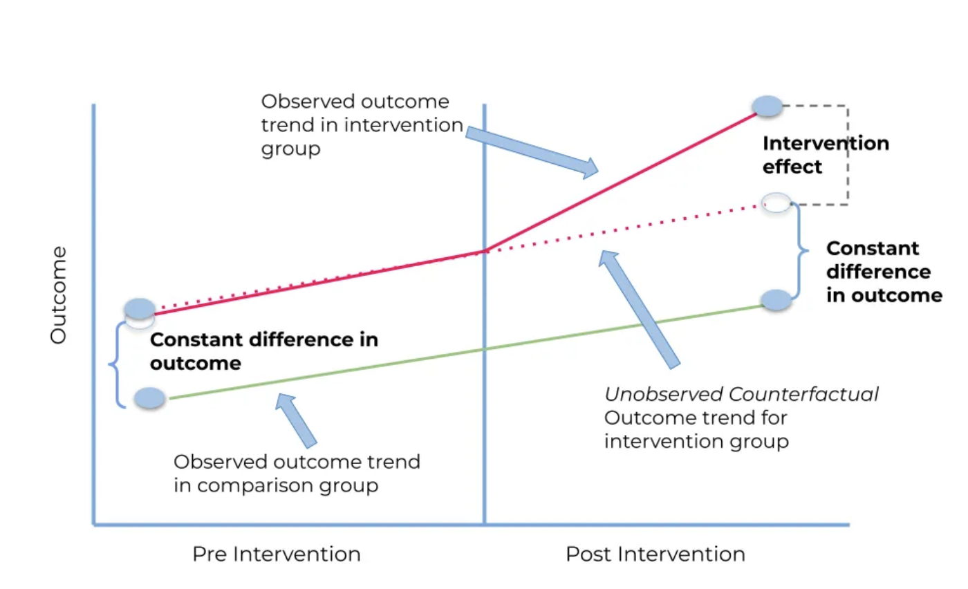
This hierarchy is fundamental. The RCT sits at the top because randomization is the most powerful tool we have for establishing causation. But notice that I'm not saying RCTs are always the best choice — sometimes they're unethical, impractical, or unnecessary. Quasi-experimental designs like difference-in-differences can be very powerful when randomization isn't feasible. The key is understanding what assumptions each design requires and whether those assumptions are plausible in your context.

The Counterfactual & Potential Outcomes

Six months after distribution, 7-day diarrhea prevalence among children under 5 is 8.7%. Is that good or bad?

You cannot answer without knowing what the prevalence would have been without the intervention. This unobservable quantity is the counterfactual.

If counterfactual = 13%

29% reduction. Scale nationally.

If counterfactual = 8%

No effect. Don't waste resources.

The Potential Outcomes Framework (Neyman-Rubin)

For each child i: Y_i(1) = outcome if treated; Y_i(0) = outcome if not treated.

Causal effect = Y_i(1) − Y_i(0). The fundamental problem: we can only observe ONE potential outcome per child.

Average Treatment Effect (ATE) = E[Y_i(1)] − E[Y_i(0)]. Randomization makes the control group an unbiased estimate of the treated group's counterfactual.

This is the deepest idea in causal inference. You observe 8.7% diarrhea prevalence among children who received the intervention. Is that good? You literally cannot answer that question without knowing the counterfactual — what would have happened without the intervention. The fundamental problem is that we can never observe both potential outcomes for the same child. That's why we need a control group: it serves as our best estimate of what the treated group's outcome would have been without treatment.

Why Randomization Solves Confounding

Randomization ensures that, on average, treatment and control groups are identical in every way except the intervention — including unmeasured confounders.

What Randomization Gives You

Exchangeability (no confounding) • Unbiased ATE estimation • Valid statistical inference • Transparent, pre-specified analysis

What It Does NOT Give You

Protection from attrition bias • Protection from measurement bias • External validity / generalizability

Intention to Treat (ITT)

The ATE of being assigned to treatment, regardless of compliance. In Rwanda: the effect of living in a sector that received filters — not the effect of actually using the filter. ITT is the primary estimand for RCTs.

Rwanda Trial: Randomization at the sector level balanced observed covariates (age, sex, water source, sanitation type).

Randomization is powerful because it balances both measured and unmeasured confounders between groups. But notice what it does NOT protect you from — attrition bias and measurement bias can still wreck your trial even with perfect randomization. Also pay attention to the ITT principle: we analyze by assigned group, not by actual use. In Rwanda, we estimate the effect of living in a sector that received filters, regardless of whether each household actually used the filter. That's the real-world policy-relevant question.

Individual vs. Cluster Randomization

Individual Randomization

Each person randomly assigned. Gold standard for independence. Problem: impractical for community-level interventions.

Cluster Randomization

Groups (villages, sectors) randomized. Prevents contamination. Cost: fewer independent units = less power. Requires GEE or mixed models.

Rwanda Trial: 96 sectors cluster-randomized 3:1. Sectors contain ~40 villages each. Stratified by district (7 districts). 3:1 ratio driven by programmatic goal of reaching 75% of the province in year 1.

Rwanda Trial: Two Studies in One

Sector-Level Study (Population Scale)

All ~82,000 children < 5 in 96 sectors. Data from health facility records and CHW reports.

Village-Level Sub-Study (Intensive Data)

174 village clusters, 1,582 households. 1:1 ratio via PPES sampling. Surveys, water sampling, PM_2.5 monitoring, sensors.

Design lesson: When feasible, nest an intensive sub-study within a larger pragmatic trial.

In Rwanda we couldn't randomize individual households — if your neighbor gets a filter and you don't, there's contamination and resentment. So we randomized at the sector level, which means entire administrative units got the intervention or didn't. The cost is statistical: with only 96 clusters, you have far fewer independent units than if you'd randomized 5,000 individual households. We also nested an intensive village-level sub-study within the larger trial, which gave us the detailed sensor and water quality data alongside the population-level health outcomes.

Randomization vs. Random Sampling

Two distinct uses of randomness serving fundamentally different purposes.

Random Sampling

Purpose: Select who enters the study
Protects: External validity (generalizability)
Threat if absent: Results may not generalize

Randomization (Random Allocation)

Purpose: Assign who receives treatment
Protects: Internal validity (causal inference)
Threat if absent: Confounding

	With Randomization	Without Randomization
With Sampling	Strongest: causal + generalizable (rare)	Generalizable, not causal (e.g., DHS)
Without Sampling	Causal, limited scope (most RCTs, e.g., Tubeho Neza)	Weakest: neither causal nor generalizable

Key insight: Most trials have randomization without random sampling — establishing causation within a specific context.

Students often confuse these two concepts, and it's worth being precise. Random sampling is about who gets into the study — it protects external validity. Randomization is about who gets the treatment — it protects internal validity. The Rwanda trial had randomization but not random sampling of the population. That means we can make strong causal claims within Western Province, but generalizing to other contexts requires additional reasoning. Most RCTs in global health are in that bottom-left cell of the table.

Stratification & Quasi-Experimental Designs

Stratified Randomization

Ensures treatment/control balance on key variables. With only 96 clusters, pure randomization could produce imbalanced groups. Stratifying by district (7 districts) ensures proportional representation. Restricted randomization: generate many allocations, reject those with poor covariate balance.

Difference-in-Differences (DiD)

Compare change over time in treated vs. untreated groups. ΔTreated − ΔControl = causal effect. Key assumption: parallel trends — both groups would have followed the same trajectory without intervention.

Other Quasi-Experimental Designs

Regression Discontinuity (RDD): Exploit an eligibility cutoff. Households just above/below the Ubudehe threshold are similar but one gets the intervention. Estimates local effect at the cutoff.
Interrupted Time Series (ITS): Track outcomes over time; look for level/slope change at intervention point. Requires long pre-intervention series (8+ data points).

With 96 clusters, pure randomization could produce imbalanced groups just by chance. Stratifying by district ensured that each district had proportional representation in treatment and control arms. I also want you to know about quasi-experimental designs because you won't always be able to randomize. Difference-in-differences is especially useful — it controls for time-invariant confounders by comparing changes over time between groups. The key assumption is parallel trends, meaning both groups would have followed the same trajectory absent the intervention.

Research Methodology

Measurement & Statistics

Now we shift from study design to the nuts and bolts of measurement and statistics. Good design means nothing if your instruments are unreliable or your analysis is inappropriate. We'll cover how to assess measurement quality, the key disease frequency measures, and then the statistical tools you need to analyze trial data properly.

Reliability & Validity of Measurement

Any measurement instrument must demonstrate both before its data can be trusted.

Reliability (Consistency)

A reliable instrument yields the same result repeatedly. Necessary but not sufficient — consistent measurement can still be consistently wrong.

Types: Test-retest (ICC, Pearson r) • Inter-rater (Cohen’s κ) • Intra-rater (ICC) • Internal consistency (Cronbach’s α)

Validity (Accuracy)

A valid instrument measures the construct it claims to measure. Without validity, reliability is meaningless.

Types: Content (expert panels) • Criterion (sensitivity/specificity, AUC-ROC) • Construct (CFA, convergent/discriminant)

Key Metrics

Metric	Range	Poor	Moderate	Good	Excellent
ICC	0–1	< 0.50	0.50–0.75	0.75–0.90	> 0.90
Cohen’s κ	−1 to 1	< 0.20	0.21–0.60	0.61–0.80	> 0.80
Cronbach’s α	0–1	< 0.60	0.60–0.70	0.70–0.90	> 0.90

Before we trust any data, we need to know whether our instruments actually work. Reliability asks whether the measurement is consistent — do you get the same result each time? Validity asks whether it's accurate — are you measuring what you think you're measuring? The key insight is that reliability is necessary but not sufficient. A scale that consistently reads two pounds too heavy is reliable but not valid. These metrics in the table are your benchmarks for evaluating any measurement tool.

How Reliability & Validity Interact

Low R, Low V

Scattered, off-center. Needs complete redesign.

High R, Low V

Tightly clustered, off-center. Most deceptive: looks precise but systematically wrong.

Low R, High V

Scattered around center. On average correct but too noisy. Increase sample size.

High R, High V

Tightly clustered on center. The gold standard.

Pitfalls: Assuming reliability implies validity • Validating in one population but applying in another • Reporting only Cronbach’s α without factor structure

Think of this like a target analogy. High reliability with low validity means your shots are tightly clustered but off-center — that's the most dangerous scenario because it looks precise but is systematically wrong. In the Rwanda trial, self-reported filter use was highly reliable across enumerators but not valid when compared to sensor data. The lesson is that you always need to validate your instruments against an objective reference standard, and a validation done in one population may not transfer to another.

Disease Frequency: Incidence & Prevalence

Building on the introduction in the Epidemiology section — here we formalise the mathematical framework.

Incidence: New Cases Over Time

Cumulative incidence (risk): New cases / Population at risk at start. e.g., 50/500 = 10% over 6 months
Incidence rate: New cases / Person-time at risk. e.g., 50/250 person-years = 0.20/person-year. Accounts for variable follow-up.

Person-time: A child observed 6 months contributes 0.5 person-years.

Prevalence: Proportion with Disease

Point prevalence: Cases at one time / Total population. A snapshot mixing new and ongoing cases.
Period prevalence: Cases during a period / Population. "Has your child had diarrhea in the past 7 days?"

Prevalence = Incidence × Duration. Treatment that shortens episodes reduces prevalence without changing incidence.

Rwanda Trial: Primary outcome was 7-day period prevalence of caregiver-reported diarrhea and ARI. Repeated cross-sectional visits at ~4-month intervals.

Incidence and prevalence are the two fundamental measures of disease frequency, and confusing them is a common mistake. Incidence counts new cases over time — it tells you the rate at which people get sick. Prevalence is a snapshot of how many people are currently sick. The relationship between them is elegant: prevalence equals incidence times duration. In the Rwanda trial, our primary outcome was 7-day period prevalence, which is a practical compromise — asking caregivers about the past week captures recent illness while minimizing recall bias.

Measures of Association: Relative & Absolute

Relative Measures

Rwanda Trial primary estimand: Prevalence Ratio from log-binomial GEE.

Values < 1 indicate a protective effect; > 1 indicates increased risk.

Absolute Measures

Risk/Prevalence Difference: RD = Risk(exposed) − Risk(unexposed). Rwanda diarrhea: 8.7% − 12.9% = −4.2 percentage points
Number Needed to Treat: NNT = 1/|RD|. Rwanda: 1/0.042 ≈ 24 households per case prevented in a 7-day window

Relative measures tell you how strong the effect is. Absolute measures tell you how much disease you actually prevent. Always report both.

A prevalence ratio of 0.71 for diarrhea means a 29% reduction — that's the relative measure. But what does that mean in absolute terms? The prevalence difference was about 4.2 percentage points, which translates to a number needed to treat of about 24 households per case prevented in any given week. Policymakers need both numbers. A 50% relative reduction sounds impressive, but if the baseline risk is tiny, the absolute benefit may not justify the cost. Always report both relative and absolute measures.

Self-Report vs. Sensor & Evaluation Design

Filter use declined: 75.5% → 67.6% → 64.8%. Traditional stove use increased: 24.1% → 49.4% ("stove stacking").

Implications for Evaluation Design

Triangulate: Self-report + observation + sensor + biomarker. Avoid reliance on a single method.
Negative controls: Include outcomes that shouldn't be affected (Rwanda: toothache). If treatment reduces toothache, you have a bias problem.
Blinding matters: Unblinded trials with subjective outcomes overestimate effects. Pooled masked HWT trials found no significant effect on diarrhea.
Plan measurement validation: Budget for sensor sub-studies and spot-checks — these are essential, not extras.

The best study design in the world is undermined by poor measurement.

This slide gets at one of the most important findings from the Rwanda trial. Self-reported filter use was nearly double the sensor-confirmed rate. That's not just noise — it's systematic overestimation driven by social desirability bias. We also used negative control outcomes like toothache: if the intervention appears to reduce toothache, something is wrong with your measurement, not your intervention. And the point about blinding is critical — pooled analyses of blinded water treatment trials found no significant effect on diarrhea, which suggests that unblinded self-report overestimates treatment effects.

The Core Problem of Statistical Inference

We want to learn about a population, but we can only observe a sample.

Population

Parameters (fixed, unknown): True mean diarrhea prevalence across all children under 5 in Western Province, Rwanda

Sample

Statistics (variable, calculated): Observed prevalence of 8.7% from a survey of 2,000 households in 30 randomly selected villages

Key Concepts

Sampling distribution: Distribution of a statistic across all possible samples of the same size
Central Limit Theorem: Sampling distribution of the mean approaches normal as n increases
Standard error: SD of the sampling distribution — measures estimate precision. Larger samples → smaller SEs

Key intuition: Probability distributions let us quantify uncertainty — which results would be common vs. surprising given a particular assumption.

This is the foundational problem of all statistics. We want to know the true diarrhea prevalence for all children under 5 in Western Province — that's the population parameter. But we can only measure a sample. The central limit theorem tells us that if we took many samples, the distribution of their means would be approximately normal, and the standard error tells us how spread out those sample means would be. Larger samples give smaller standard errors, which means more precise estimates. This is the machinery behind every confidence interval and hypothesis test we'll discuss.

The Logic of Hypothesis Testing

1. Assume No Effect

H₀: Filter distribution has no effect on diarrhea prevalence.

2. Calculate Expected

Under H₀, how much would prevalence vary between groups by chance?

3. Compare Observed

You observed a 4.3 pp difference. Test statistic t = 3.7.

4. Quantify Surprise

p = 0.002. Only 0.2% of random samples would show this large a difference.

Proof by contradiction: assume no effect exists, show the data would be very unlikely under that assumption, conclude the effect is probably real.

Two Ways to Be Wrong

	Reality: H₀ TRUE	Reality: H₀ FALSE
Reject H₀	Type I Error (α) — false positive	Correct (Power = 1 − β)
Fail to reject	Correct (true negative)	Type II Error (β) — false negative

Hypothesis testing is really proof by contradiction. We start by assuming the null — that our intervention has no effect. Then we ask: if there truly were no effect, how surprising would our observed data be? In the Rwanda trial, the observed difference was large enough that it would occur by chance only 0.2% of the time under the null — that's highly surprising, so we reject the null. The two-by-two table of errors is critical: a Type I error means we claim an effect that doesn't exist, and a Type II error means we miss an effect that does. Power is our ability to detect a real effect.

P-Values & Confidence Intervals

The Epi section introduced CI interpretation and NNT. Here we examine what p-values actually mean — and what they do not.

What the P-Value IS

The probability of observing data at least as extreme as your result, assuming H₀ is true. p = 0.03 means: if there were truly no effect, you'd see this result only 3% of the time.

What the P-Value is NOT

NOT the probability that H₀ is true
NOT the probability of a false positive
NOT a measure of effect size

α = 0.05 is a convention, not a law. Some fields use 0.01 or 0.10. Set before analyzing data.

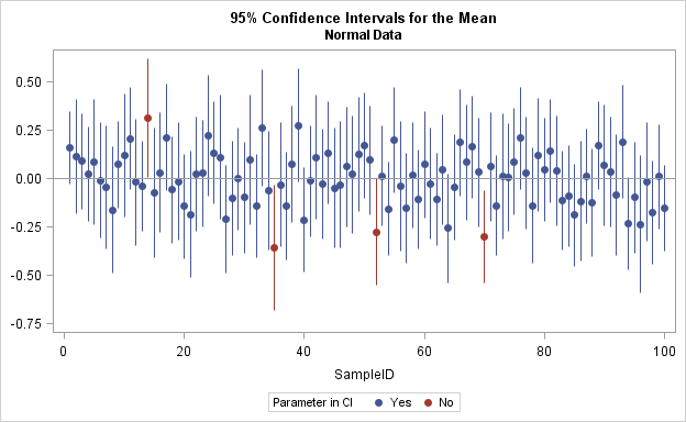
Confidence Intervals: Beyond Yes/No

If you repeated your study 100 times and computed a 95% CI each time, approximately 95 of those intervals would contain the true parameter. CIs provide the range of plausible effect sizes.

P-values are the most misunderstood concept in statistics. A p-value of 0.03 does NOT mean there's a 3% chance the null is true — it means that if the null were true, you'd see data this extreme only 3% of the time. That's a subtle but important distinction. I strongly prefer confidence intervals because they give you more information — not just whether an effect exists but how big it might plausibly be. A confidence interval that is narrow and excludes the null tells you much more than a single p-value ever could.

Choosing the Right Statistical Test

Before choosing a test, answer three questions: (1) What is your outcome variable? (2) How many groups? (3) Are assumptions met?

Outcome	Scenario	Parametric	Non-Parametric
Continuous	1 sample vs. known value	One-sample t-test	Wilcoxon signed-rank
	2 independent groups	Independent t-test	Mann-Whitney U
	3+ groups	One-way ANOVA	Kruskal-Wallis
Categorical	2×2 independent	Chi-square test (Fisher’s exact if cell < 5)
	Paired before/after	McNemar’s test
	Multiple predictors	Logistic regression
Time-to-event	Estimate/compare curves	Kaplan-Meier / Log-rank test
Time-to-event	Model with covariates	Cox proportional hazards regression

Go non-parametric when: n < 30 and non-normal • Skewed data (income, costs) • Ordinal scales (Likert, staging)

This table is your reference guide for choosing the right statistical test. The decision process is straightforward: first identify your outcome variable type — continuous, categorical, or time-to-event. Then ask how many groups you're comparing, and whether parametric assumptions are met. For the Rwanda trial, we had a binary outcome — diarrhea yes or no — so we're in the categorical row, and because we needed to model covariates and account for clustering, we used GEE regression rather than a simple chi-square test.

Correlation, Regression & Survival Analysis

Correlation

Pearson’s r: Both continuous and normal. Linear relationship. e.g., income vs. water quality
Spearman’s rho: Ordinal or non-normal. Monotonic relationship. e.g., education level vs. health knowledge rank

Regression

Linear regression: Continuous outcome. Y = b₀ + b₁X + e. e.g., predict child BMI from diet and activity
Logistic regression: Binary outcome. Log-odds as linear function. e.g., predict diarrhea Y/N from WASH variables
Poisson / Negative binomial: Count outcome. Rate of events per unit time. e.g., clinic visits per month

Survival Analysis

Kaplan-Meier: Estimate survival curves. Handles censoring
Log-Rank test: Compare survival between 2+ groups
Cox regression: Model hazard with covariates. Produces hazard ratios

These are the workhorses of quantitative analysis. Correlation tells you about the strength and direction of a relationship but not causation. Regression lets you model outcomes as a function of multiple predictors — linear regression for continuous outcomes, logistic for binary, Poisson for counts. Survival analysis is what you use when you're tracking time until an event and some participants haven't experienced the event yet — that's called censoring. Cox regression is especially powerful because it lets you model hazard rates while adjusting for covariates.

Statistical Test Decision Tree

What is your outcome variable?

Continuous

1 sample → t-test / Wilcoxon
2 groups → t-test / Mann-Whitney
3+ groups → ANOVA / Kruskal-Wallis
Paired → Paired t / Wilcoxon

Categorical

Independent → Chi-square / Fisher’s
Paired → McNemar’s test
Model → Logistic regression

Time-to-Event

Estimate → Kaplan-Meier
Compare → Log-rank test
Model → Cox regression

Quick Rules of Thumb

Continuous outcome + 2 groups → start with a t-test
Binary outcome → chi-square for comparison, logistic regression for modeling
Censored follow-up time → survival analysis (Kaplan-Meier, log-rank, Cox)
Clustered data → mixed models or GEE, not standard tests

This decision tree is a visual summary of the previous slide. Start with your outcome variable type, then follow the branches. The last rule of thumb is the most important one for this course: if you have clustered data — and you almost always do in global health research — you cannot use standard tests. You need mixed models or GEE. I've seen published papers in major journals that ignore clustering, and their conclusions are wrong because of it. We'll get into that next.

Research Methodology

Advanced Topics

Clustering, Missing Data & Generalizability

These are the topics that separate competent analysis from naive analysis. Clustering, missing data, and generalizability are the three issues that trip up most researchers in global health. If you don't handle them properly, your results could be seriously misleading — and many published studies get this wrong.

Rwanda Trial: Primary Analysis in Detail

The Analytic Pipeline

Outcome: Binary (diarrhea yes/no in past 7 days)
Model: Log-binomial regression → directly estimates prevalence ratio
Clustering: GEE with exchangeable working correlation, robust (sandwich) SEs at village level
Covariates: Child age (months) and sex only — minimal adjustment since randomization handles confounding
Weights: Sampling weights to account for PPES design in village-level sub-study

Water quality improved significantly. Air quality did not — consistent with stove stacking behavior detected by sensors.

Let me walk you through exactly how we analyzed the Rwanda trial data. We used log-binomial regression because it directly estimates prevalence ratios, which is what we wanted. We used GEE with robust standard errors to account for clustering at the village level, and we only adjusted for child age and sex — minimal adjustment because randomization should handle confounding. Look at those results: significant reductions in diarrhea, ARI, and water contamination, but no effect on air quality. That null result for PM2.5 is consistent with the stove stacking behavior the sensors detected.

The Issue of Clustering

Children within the same village share water sources, sanitation, disease ecology, climate, economic conditions, CHW quality, and health facility access. Their health outcomes are correlated — not independent.

Intraclass Correlation & Design Effect

ICC = σ²(between) / [σ²(between) + σ²(within)] — proportion of variance due to between-cluster differences.

Design Effect (DEFF) = 1 + (m − 1) × ICC, where m = average cluster size. Effective sample size = n / DEFF.

Level	Outcome	ICC	Design Effect
Within-village	Diarrhea	0.02	1.18 (m=10)
Within-village	ARI	0.04	1.36 (m=10)
Sector-level	Diarrhea	—	9.5
Within-child (repeated)	Diarrhea	0.09	—

Clustering is probably the single most important statistical concept for global health research. Children in the same village share water sources, sanitation facilities, the same community health worker — their outcomes are correlated. The ICC tells you what fraction of the total variance is between clusters versus within clusters. Even an ICC of 0.02 can produce a design effect of nearly 10 at the sector level, meaning your effective sample size is a tenth of what you think it is. This has enormous implications for how we design and analyze studies.

Ignoring Clustering & Sample Size

What Happens When You Ignore Clustering

If you analyze 5,000 children from 10 clusters as independent observations, your nominal 5% significance level may actually be 20–30%. This is one of the most common methodological errors in global health research.

Sample Size Under Clustering

The number of clusters matters more than individuals per cluster.

Clusters needed per arm: k = (Z_α + Z_β)² × DEFF × 2σ² / δ². Adding more people per cluster gives diminishing returns once m × ICC > 1.

Better to have 20 clusters of 50 than 10 clusters of 100. Always calculate cluster-adjusted sample sizes.

Here's what happens when you ignore clustering: your false positive rate explodes. If you treat 5,000 children from 10 clusters as independent observations, your nominal 5% significance level might actually be 20 or 30 percent. The practical lesson for study design is that the number of clusters matters far more than the number of individuals per cluster. It's always better to have more clusters with fewer people each than fewer clusters with more people. This is counterintuitive but mathematically inevitable once outcomes are correlated within clusters.

100

Analytic Solutions for Clustering

Cluster-Robust SEs

"Sandwich" standard errors. Inflate SEs to account for within-cluster correlation. Requires ≥30 clusters. Simplest solution.

GEE

Generalized Estimating Equations. Specify working correlation structure. Robust SEs protect against misspecification. Population-averaged. Used for Rwanda primary analysis.

Mixed Models

Random effects / multilevel models. Estimate cluster-specific parameters. Handle multiple nesting levels. Cluster-specific interpretation.

For policy questions ("what’s the average effect?"), GEE is preferred. For prediction ("what will happen in this village?"), mixed models are preferred.

Rwanda Trial: GEE with exchangeable working correlation and robust SEs, clustering at village level.

So how do we actually handle clustering? These are your three main options. Cluster-robust standard errors are the simplest — they inflate your standard errors to account for within-cluster correlation, but you need at least 30 clusters. GEE is what we used in the Rwanda trial — it's a population-averaged approach that gives you the average effect across all clusters. Mixed models give you cluster-specific estimates, which is useful if you want to predict outcomes for a particular village. The choice between GEE and mixed models depends on your research question: policy questions favor GEE, prediction questions favor mixed models.

101

Missing Data Mechanisms

Rubin’s classification defines why data are missing — and determines which analytic methods are valid.

MCAR — Least Concern

Missingness unrelated to any data. Loss of power but no bias. Complete-case analysis valid.

e.g., Lab machine randomly malfunctions

MAR — Moderate Concern

Missingness depends on observed data. Biased if ignored. Recoverable with MI or ML methods.

e.g., Younger participants miss follow-up

MNAR — Greatest Concern

Missingness depends on the unobserved value itself. Biased under all standard methods. Requires sensitivity analyses.

e.g., Depressed patients don’t complete depression scale

Missing data is unavoidable in field research — people move, refuse to participate, or are simply not home when the enumerator visits. Rubin's classification of missing data mechanisms tells you which analytic methods are valid. MCAR is the easiest case — data are randomly missing and you just lose power. MAR is the common case where missingness depends on something you've measured, like age or location. MNAR is the nightmare scenario — the sickest children are the ones you can't find, and no standard method can fully correct for that.

102

Analytic Solutions for Missing Data

Method	Valid Under	How It Works
Complete-Case Analysis	MCAR	Delete cases with missing values. Simple but wasteful. Biased unless MCAR.
Single Imputation	MCAR	Replace with mean/median/LOCF. Underestimates variance. Rarely recommended.
Multiple Imputation (MI)	MAR	Create m complete datasets (20–50) with plausible imputed values. Pool results via Rubin’s rules.
Maximum Likelihood (ML)	MAR	Estimate parameters directly from observed data likelihood (EM, FIML). No imputed datasets needed.
Inverse Probability Weighting	MAR	Weight complete cases by inverse probability of being observed. Combines with MI for doubly robust estimation.
Sensitivity Analysis	MNAR	Vary assumptions about missing values. Pattern-mixture models, selection models, tipping-point analyses.

This table gives you the toolkit for handling missing data. The key message is: never just delete cases with missing values unless you're confident the data are MCAR, which is rare. Multiple imputation is usually the best approach for MAR data — you create many plausible complete datasets, analyze each one, and pool the results. For MNAR, the honest answer is that no method can fully fix the problem, so you do sensitivity analyses to see how much your conclusions change under different assumptions about why data are missing.

103

External Validity: Not All Water Treatment Works

Randomized trials of chlorination in Bangladesh, Kenya, and Zimbabwe found NO significant effect on childhood diarrhea.

Pathogen Profile

Chlorine is ineffective against Cryptosporidium. LifeStraw removes it through physical ultrafiltration. Intervention type matters.

Measurement & Blinding

Chlorination trials with blinded outcomes (sham chlorine) found no effect. Unblinded self-reported outcomes may overestimate effects.

The generalizability question isn’t "does water treatment work?" It’s "which treatment, against which pathogens, in which context, with what delivery model?"

Internal vs. External Validity

The Rwanda trial has strong internal validity (cluster-RCT, pre-registered, large sample). But results are specific to: Western Province, Rwanda | Poorest quartile | Rural | LifeStraw + EcoZoom | CHW-delivered with carbon credit financing.

This is one of the most important slides in the course. Rigorous RCTs of chlorination in multiple countries found no effect on diarrhea. Does that mean water treatment doesn't work? No — it means the specific intervention, against the specific pathogen profile, in the specific context, didn't work. Chlorine doesn't kill Cryptosporidium, but a physical filter like LifeStraw removes it. And when blinded trials with sham chlorine found no effect, it suggested that prior unblinded results were inflated by courtesy bias in self-reported outcomes. The question is never "does water treatment work" in the abstract — it's always context-specific.

104

Effect Modification: Why Effects Vary

Treatment effects are not universal constants. They vary across subgroups and contexts.

Biological Modifiers

Age: children < 2 more susceptible
Nutritional status
HIV/immune status
Pathogen profile: filter vs. chlorine

Contextual Modifiers

Baseline water quality
Baseline disease burden
Competing transmission routes

Implementation Modifiers

CHW network quality
Supply chain reliability
Cultural acceptability
Government support

Always report subgroup analyses and discuss which modifiers might limit transportability. Rwanda’s strong CHW system is unusual — replication elsewhere may yield smaller effects.

Treatment effects are not universal constants — they depend on who receives the intervention and under what conditions. Biological modifiers like age and nutritional status change how children respond. Contextual modifiers like baseline water quality determine how much room there is for improvement. And implementation modifiers like the quality of the CHW network can make or break an intervention. Rwanda has one of the strongest community health worker systems in Africa — replicating these results in a country with a weaker health system might yield smaller effects, and you need to be honest about that in your discussion section.

105

Efficacy → Effectiveness → Scale

Why Effects Shrink at Scale

Adherence: Self-reported filter use declined 75.5% → 64.8%. Sensor data: actual use ~37%.
Stove stacking: Traditional fire use increased 24.1% → 49.4%. No exclusive adoption → no air quality improvement.
Implementation variation: Hundreds of CHWs with varying training, supply chain delays, seasonal access challenges.

This is the sobering reality of scaling interventions. In controlled pilot conditions with supervised use, the LifeStraw filter achieved 97.5% reduction in thermotolerant coliforms. At scale in the real world, that dropped to 38%. That's a 2.5-fold gap between efficacy and effectiveness. Adherence declined over time, stove stacking meant traditional fires persisted alongside the improved cookstove, and implementation varied across hundreds of community health workers. This is why I keep emphasizing that what works in a pilot may not work at scale — and why sensor-based monitoring of actual use is so critical.

106

Key Takeaways

Health is shaped by systems

Determinants of health extend far beyond healthcare — water, sanitation, air quality, governance, and poverty all drive disease burden.

Measurement matters

Self-report ≠ reality. Sensors, objective measurement, and rigorous study design are essential to understanding what actually works.

Efficacy ≠ effectiveness

Interventions that work in trials often fail at scale. Adherence, implementation fidelity, and local context determine real-world impact.

Engineers build the solutions

Water filters, sensors, surveillance systems, and monitoring infrastructure — engineering is where global health evidence becomes action.

Let me leave you with four things I hope you take away from this course. First, health is shaped by systems — not just healthcare, but water, sanitation, air quality, governance, and poverty. Second, measurement matters — self-report is not reality, and we need sensors and rigorous study design. Third, efficacy does not equal effectiveness — what works in a pilot often fails at scale. And fourth, engineers build the solutions. The evidence base we've been discussing all semester is only useful if someone designs and deploys the technologies, the monitoring systems, and the infrastructure that translate knowledge into health impact.

107

Lab Assignment

Global Burden of Disease Lab

Water quality QMRA & air quality cost-effectiveness analysis using R, GBD Compare, and HAPIT.

Open Full Lab Assignment →

For your lab assignment, you'll be working hands-on with the Global Burden of Disease data tools and doing two analyses. The first is a quantitative microbial risk assessment for water quality, and the second is a cost-effectiveness analysis for air quality interventions using HAPIT. You'll use R for the analysis and GBD Compare to contextualize your findings. Click the link to open the full assignment with detailed instructions.

Global Health for Engineers

Course Structure

Evan Thomas

The Global Health Architecture

The Current State of Global Health

USAID Shutdown

US Withdrawal from the WHO

EPA Rollbacks, CDC Cuts & Domestic Health

Implications for Global Health Engineers

Intro to Global HealthPart 1 - Overview

What is Global Health?

Disease & Determinants of Health

Multi-sectoral Dimension of the Determinants of Health

One Health — Zoonotic Disease at the Human-Animal-Environment Interface

Governance & Armed Conflict

Intro to Global HealthPart 2 – Global Burden of Disease

Explore the Data

Health & Income of Nations

Global Mortality Among Children Under 5

Child Mortality in Sub-Saharan Africa

Extreme Poverty by Region

Per Capita CO2 Emissions

Global Burden of Disease

Undernourishment

Child Mortality — Causes of Death Under 5

Communicable & Non-Communicable Diseases

Communicable Diseases — Definition & Transmission

Impact of Communicable Diseases

Malaria

Malaria Control

HIV/AIDS Infections Over Time

Global HIV Burden

HIV/AIDS

Non-Communicable Diseases (NCDs)

Air Quality and Public Health

Water and Public Health

Sanitation and Public Health

Epidemiology & Biostatistics

John Snow & the Birth of Epidemiology

Epidemiology — Defined

Epidemiology Key Terms

Incidence vs. Prevalence

Measurement of Health Status

Understanding Dose-Response Curves

Dose-Response: Clean Drinking Water

Dose-Response: Air Pollution Exposure

Modern Scenario: COVID-19 Outbreak Investigation

Epidemiology Study Types

Confounding

Measuring the Association between Exposure and Outcome

Epidemiological Formulas

Worked Example: Odds Ratio

Sensitivity & Specificity

Confidence Intervals, p-values & NNT

Public Health Interventions

Digital Epidemiology — Engineering Tools for Disease Surveillance

Surveillance & Public Health Approach

Approaches to Interventions

Behavior Change

Randomized Controlled Trial (RCT)

Cost-Effectiveness Analysis

Implementation Science

Health System Strengthening

Rwanda Tubeho NezaWater Filter & Cookstove Programme

Rwanda — Country Context

Programme Implementation

Key Results — Tubeho Neza Trial

Technology & Digital Monitoring

Water Filters

Remote Sensing Innovation

Carbon Credit Model

Scale, Carbon Finance & Lessons Learned

Published Research (13 Papers)

From Research to Methodology

Research Methodology

Applying Methodology to Tubeho Neza

Biased Approaches to Evaluation

Biased Approach #1: Before vs. After

Biased Approach #2: Users vs. Non-Users

The Three Systematic Threats to Validity

Intro to Global Health
Part 1 - Overview

Intro to Global Health
Part 2 – Global Burden of Disease

Per Capita CO₂ Emissions

Rwanda Tubeho Neza
Water Filter & Cookstove Programme